Key Concepts

This page collects the ideas hensmith implements: what a minimum approach temperature is, how the problem table turns a set of process streams into utility targets and a pinch, how synthesize_network() turns those targets into a network of exchangers, and what the result is and is not guaranteed to be. Everything below describes the behavior of the code in hensmith/hxn_synthesis.py and hensmith/_heat_exchanger_network.py, and of their two private helpers, hensmith/_curves.py (the stream curves) and hensmith/_planner.py (the network planner); the Tutorial shows the same concepts on a running system.

Heat integration and the minimum approach temperature

Every heating and cooling duty in a flowsheet is paid for with a utility: steam, cooling water, chilled water, refrigerant. Heat integration replaces part of that spending with process-to-process exchange – heat taken from a stream that must be cooled and given to a stream that must be heated. What is left after the process exchangers have done as much as they can is the irreducible utility demand.

Heat only flows down a temperature gradient, and a finite exchanger can only transfer heat across a finite temperature difference: the closer the two streams are in temperature, the more area is needed for the same duty, since the area of a counter-current exchanger scales as \(Q / (U \Delta T_{lm})\). hensmith expresses that limit as a single number, the minimum approach temperature T_min_app (in K, default 5.), used to shift hot streams in the problem table and required between the streams everywhere inside every synthesized exchanger:

• in problem_table(), where every hot stream’s temperature is shifted down by T_min_app before the streams are compared, so that two streams which meet on the shifted scale are really T_min_app apart;

• in the planner of synthesize_network(), which admits a match only if the two streams stay at least T_min_app apart at every breakpoint of their temperature-enthalpy curves along the whole exchanger, not only at its two ends; and

• on every synthesized process exchanger, whose approach is verified on the exact states of its two streams, again along its whole length. The exchanger itself is a biosteam.HXprocess constructed with dT=T_min_app - 1e-6, a guard against rounding only.

Lowering T_min_app lowers the utility targets and raises exchanger area; raising it does the reverse. It is the parameter in hensmith that sets the trade between utilities and capital, and because HeatExchangerNetwork reports its capital as added cost and its utilities as differences (see below), both sides of that trade are visible in the facility’s results.

Shifted temperatures and the problem table

problem_table() builds the temperature-interval heat cascade of a set of streams, given each stream’s inlet, its outlet quenched to equilibrium at its own enthalpy, a flag saying whether it is cooled, and T_min_app. Its result is a ProblemTable.

Stream curves. Each stream is first described by a piecewise-linear temperature-enthalpy curve over its own enthalpy range, built once from a handful of flashes and evaluated afterwards without flashing. Its breakpoints are the stream’s two end temperatures and every phase boundary inside its range (a pure component’s saturation temperature, a mixture’s bubble and dew points); a pure component’s latent heat is a flat (isothermal) segment between its saturated-liquid and saturated-vapor enthalpies; a mixture’s two-phase glide is sampled, and so is every curved single-phase stretch (temperature-dependent heat capacity), densely enough that linear interpolation stays within 0.002 K of the true curve. Inside its range the stream is taken at equilibrium with its enthalpy clipped to \([H_{lo}, H_{hi}]\), so a stream copy at an interior temperature can never carry more enthalpy than the real stream ever has (a non-equilibrium outlet, for instance); what a non-equilibrium end state departs from equilibrium at its own end temperature becomes a flat there.

The shifted grid. Hot streams are shifted down by T_min_app; cold streams are not. The grid Ts is the sorted (descending) union of the shifted breakpoints of all curves, temperatures closer than 1e-9 K being one grid point. Every temperature at which any stream’s curve bends or jumps is therefore a grid point, and between two consecutive grid points every stream is linear to within 0.002 K. A grid of the stream end temperatures alone would average a boiling point, a dew or bubble point, or the curvature of a glide that falls strictly inside an interval over that interval, which can hide a pinch and make the hot utility target too low.

Per-stream contributions. Write \(H_j^-(T)\) and \(H_j^+(T)\) for the low- and high-enthalpy limits of stream \(j\)’s curve at the real temperature \(T + \mathrm{shift}_j\); they differ only where the curve has a flat at that temperature, and they are \(H_{hi}\) above and \(H_{lo}\) below the stream’s range. The heat a stream contributes to the open interval between grid temperatures \(T_k\) and \(T_{k+1}\), and at the grid temperature \(T_k\) itself, are

\[\mathrm{interval\_H}[j,k] = s_j \left( H_j^-(T_k) - H_j^+(T_{k+1}) \right), \qquad \mathrm{point\_H}[j,k] = s_j \left( H_j^+(T_k) - H_j^-(T_k) \right),\]

with \(s_j = +1\) for a hot stream and \(-1\) for a cold one. The stream’s own end points are grid points selected by position rather than by a float comparison, so the contributions telescope exactly:

\[\sum_k \mathrm{interval\_H}[j,k] + \sum_k \mathrm{point\_H}[j,k] = s_j \left| H_{out} - H_{in} \right|,\]

that is, to the stream’s duty.

Point loads. point_H is nonzero only where a curve is flat: at a pure component’s (shifted) saturation temperature, which receives its latent heat; at an end temperature where a non-equilibrium end state departs from equilibrium; and at the shifted outlet temperature of a point-load stream – an isothermal stream, or one whose outlet temperature moves against its duty (a heated stream that leaves cooler than it entered, such as a reboiler outlet quenched to equilibrium) – which has no interval to occupy and puts its whole duty \(s_j |H_{out} - H_{in}|\) there.

The cascade. Starting from zero hot utility, the heat leaving grid boundary \(T_k\) (after that boundary’s point loads) is

\[\mathrm{residual}[k] = \sum_j \sum_{i \le k} \mathrm{point\_H}[j,i] + \sum_j \sum_{i < k} \mathrm{interval\_H}[j,i].\]

Feasibility must hold for the heat arriving at each boundary as well, before its point loads are applied,

\[\mathrm{arriving}[k] = \mathrm{residual}[k] - \sum_j \mathrm{point\_H}[j,k],\]

because a point source located at \(T_k\) cannot serve a sink above \(T_k\). hensmith therefore takes the elementwise minimum of the two flows; the most negative value is the deficit hot utility must make up,

\[\mathrm{hot\_util\_load} = -\min_k \min(\mathrm{residual}[k], \mathrm{arriving}[k]),\]

its first location is the pinch, and the heat left at the bottom of the cascade is the cold utility, \(\mathrm{cold\_util\_load} = \mathrm{residual}[-1] + \mathrm{hot\_util\_load}\). Whether that minimum is the arriving or the leaving flow at the pinch fixes the side of the pinch that the point loads at the pinch temperature belong to, the pinch cut.

Because every stream is linear to within 0.002 K between grid points, the grid minimum of the cascade is the true one to within 0.002 K times the sum of the heat capacity flow rates; equivalently, the targets lie between the exact targets at T_min_app minus and plus 0.004 K (approximately: the 0.002 K tolerance is established by midpoint tests). For streams of constant heat capacity the curves are exact.

Threshold problems. When that minimum is not negative – or negative by no more than 1e-9 of the total stream duty – no hot utility is needed at all. The table then reports zero hot utility and places the pinch at the top of the grid, Ts[0]. A cold utility that comes out slightly negative through rounding is absorbed back into the hot utility so that the identity

\[\mathrm{hot\_util\_load} - \mathrm{cold\_util\_load} = \sum_j \text{(stream duty)}\]

stays exact: the difference between the two targets is always the net heating demand of the whole set of streams. That identity is the table’s own consistency check – whatever the algorithm does with the cascade, it can neither invent nor destroy energy.

Targets: MER, pinch, composite and grand composite curves

The two loads returned by the table are the minimum energy requirement (MER) targets: the least hot and cold utility any network operating with this T_min_app can use. They are available before a single exchanger has been placed, which is what makes pinch analysis a targeting method – the target comes first, and the network is judged against it.

The same information can be read graphically. The composite curves plot cumulative enthalpy against temperature for all hot streams together and all cold streams together, on the real temperature scale. Where the two curves overlap horizontally, heat can pass from hot to cold: that overlap is the heat recovered by process exchange. The overhang of the cold curve at its warm end is the hot utility, and the overhang of the hot curve at its cold end is the cold utility. The place where the curves come closest vertically is the pinch, and by construction they approach no closer than T_min_app.

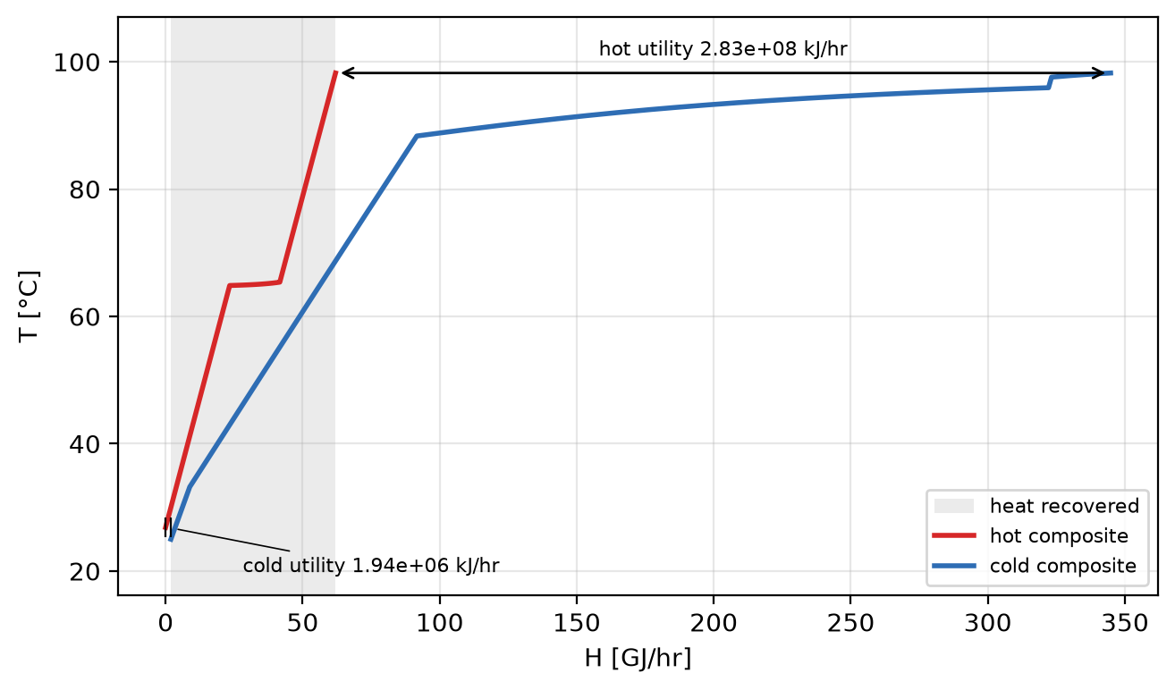
Composite curves of the quickstart system at T_min_app = 5 K. The shaded band is the heat the two curves can exchange with each other; the arrows are the two MER targets, a hot utility of 2.828e+08 kJ/hr and a cold utility of 1.936e+06 kJ/hr. The curves come closest at the cold end, where the pinch of this system lies – 298.15 K on the shifted scale. Pinch analysis and targets builds this figure from a ProblemTable.

The grand composite curve plots the same cascade differently: the heat carried through each shifted grid temperature once the minimum hot utility is supplied, against that temperature. It touches zero exactly at the pinch for a pinched problem; for a threshold problem, where no hot utility is needed, the curve’s minimum may be strictly positive and the pinch is placed at the top of the grid, Ts[0], by convention. Its shape shows where in the temperature range utility has to be added or removed.

Both pictures express the three rules of pinch design: no heat may cross the pinch, no cold utility may be used above it, and no hot utility below it. Violating any one of them makes the network use more of both utilities than the targets require, by the amount transferred across the pinch.

From targets to a network: the pinch-outward MER planner

synthesize_network() takes the heat utilities of the process, runs the problem table above, plans a network without stream splits that reaches the MER targets whenever its search finds one, and realizes the plan as BioSTEAM exchangers. Streams are numbered in a rearranged order – heated streams first, then cooled streams – and every array, exchanger ID and life cycle uses that index. The order only breaks ties in the planner’s search: the facility hands the utilities over sorted by signed duty, and sort_hus_by_T sorts them by inlet temperature instead.

The planner’s model. Each stream enters the planner as its knots on the problem-table grid: its enthalpy at every grid temperature inside its range, with two knots where its curve has a flat. Every breakpoint of every curve is a grid point and the table is linear between grid points, so the planner’s own cascade reproduces the table exactly – the same targets, the same pinch and the same pinch cut. Each stream is cut at the pinch into an above-pinch part and a below-pinch part (a stream lying wholly on one side has an empty part on the other), and the two sides are planned as two independent problems.

Must and flex streams. Above the pinch no cold utility may be used, so every hot stream there is a must: process matches have to cool it completely. The cold streams above the pinch are flex streams: whatever their matches leave over is supplied by one hot utility at their far (hot) end. Below the pinch the roles swap: no hot utility may be used, so every cold stream is a must, and the hot streams are flex streams finished by one cooler at their cold end. Putting a flex stream’s utility at its far end loses nothing: moving a stream’s later matches toward its inlet never reduces the approach of any match on it, because every stream’s curve is monotone.

Building each side from the pinch outward. A depth-first search builds each side one match at a time, starting at the pinch, where the driving forces are smallest, and moving outward. A match of duty \(x\) between a must and a flex stream is feasible only if the two streams keep T_min_app at every knot along it, so internal pinches – a condensing vapor against a boiling mixture, say – are respected, not just the exchanger’s terminals. Every step also keeps the problem table of the remaining problem feasible (remaining problem analysis): the largest duty that does so has a closed form, so no step can make MER unreachable by its own table. Wherever that remaining table is tight – a pinch of the remaining problem – the pinch design rules of Linnhoff and Hindmarsh must hold:

• above the pinch, every hot stream at the pinch needs its own cold stream at the pinch, with \(C_{hot} \le C_{cold}\) (the number rule \(N_{hot} \le N_{cold}\) and the heat-capacity-flow rule);

• below the pinch, every cold stream at the pinch needs its own hot stream at the pinch, with \(C_{hot} \ge C_{cold}\).

Both rules are generalized to isothermal segments: a flat – a pure component boiling or condensing exactly at the pinch – has unlimited series capacity and can serve several partners in turn. At the process pinch itself a violation of these rules proves that MER needs stream splitting.

The candidate duties of a match are the largest feasible one and a finite set of events: a stream is ticked off, a partner is saved for another stream, a stream switches partner or returns to an earlier one. The search is budgeted in deterministic work units rather than seconds, so its result does not depend on the speed of the machine. Once a MER plan is found, a branch and bound on the number of exchangers looks for a smaller one; consecutive pieces of the same match are merged into one exchanger.

Repeated pairs. The same hot and cold stream may be matched more than once on the same side: alternating two partners in series emulates a split, and some unsplit MER networks need it. Process exchangers are named HX_<cold>_<hot>_hs above the pinch (the hot-side design) and HX_<hot>_<cold>_cs below it (the cold-side design), the first number being the stream at port 0; the n-th exchanger of the same pair on the same side, counted in the order the hot stream meets them, gets the suffix _<n> for \(n \ge 2\) (for example HX_3_2_cs_2). Utility exchangers are Util_<index>_hs for a cold stream and Util_<index>_cs for a hot one. avoid_recycle=True forbids matching any pair twice anywhere – on one side or across the two – so that no two exchangers connect the same pair of streams, at the cost of the MER networks that need a repeated pair.

Best effort when splitting is needed. A side whose pinch rules prove that MER needs a split, or whose search runs out of budget, gets a best-effort plan instead. Heat that a must stream cannot place (a gap) is moved to the stream’s pinch end, where it crosses the pinch at the cost of an equal amount of extra hot and cold utility, the penalty; greedy dives and a bisection of the gaps keep that penalty small, though not minimal in general. Such a network reports 'best_effort'.

Small matches. A planned exchanger with a duty below Qmin (default 1e-3 kJ/hr) is dropped and its duty left to the utilities. Removing a match never reduces the approach of another, so the rest of the plan stays feasible; a large Qmin can, however, cost MER.

Realization. Each stream is walked in flow order from its inlet: a hot stream through its above-pinch matches (from its inlet end), then its below-pinch matches, then its cooler; a cold stream through its below-pinch matches, then its above-pinch matches, then its heater. Each match becomes one plain HXprocess whose two enthalpy limits, H_lim0 and H_lim1, are the planned outlet enthalpies of its two streams, so that its duty reproduces the plan. A planned outlet whose equilibrium state is not past the stream’s state at the exchanger inlet cannot be a limit (HXprocess rejects it): one strictly inside a non-equilibrium end jump, or a state of a point-load stream on the wrong side of its inlet. That stream’s limit is left out, and the other stream’s sets the duty. A stream’s first exchanger receives its real inlet – except a point-load stream, which enters at equilibrium at its inlet enthalpy, on the side of its outlet temperature where the plan put its duty – and every later exchanger receives the stream’s exact state at the planned enthalpy. Each exchanger is simulated once; one whose duty differs from the plan is reported, and one that cannot be simulated at all is dropped, its duty going to the utilities. Finally one rigorous HXutility per stream takes it to its outlet enthalpy, and an AssertionError is raised if that does not reproduce the quenched outlet enthalpy and temperature, so a network that would not deliver the specified outlets fails loudly rather than silently.

Exact approach verification. The knots are exact at grid points but are chords in between, up to 0.002 K off inside glides and curved single-phase stretches. Every planned exchanger is therefore checked on the exact states of its two streams wherever its planned approach is within that margin of T_min_app: at its ends, at every breakpoint inside it and, where the exact approach is not linear between two positions, by a search for a dip in between. HXprocess itself checks only its two terminals, which would miss an internal pinch at a phase change. Where a MER plan falls short by more than 1e-6 K, the exact states are inserted as knots and the network is planned again, for at most three rounds. A best-effort plan, or a MER plan still short after the last round, instead has each violating match shrunk to the largest duty that keeps the approach, the rest going to the utilities: with its inlets fixed, a smaller duty can only raise a match’s approach, and the later stages of both streams move toward their inlets, which never reduces another match’s approach. Streams of constant heat capacity never need either step.

The report. synthesize_network(..., info={}) fills the dictionary it is given, and HeatExchangerNetwork keeps it as synthesis_info. 'status' is 'mer' only if the utilities of the realized network, computed from the simulated exchanger duties, equal the targets (to 1e-6 of the total stream duty), and 'best_effort' otherwise. Next to it are the targets ('Q_hot_target', 'Q_cold_target'), the planned and the realized utilities, the 'penalty', per side of the pinch ('sides') the search method, its work, any proof that a split is needed and the gaps, the planner’s own targets and pinch, the number of refinement rounds, the smallest approach inside any process exchanger, the matches that were shrunk ('repaired'), dropped ('qmin_dropped', 'dropped') or deviated from their plan ('deviations'), and the point-load streams. The full list is under the info keyword of synthesize_network().

Rigor and phase change

Process streams in a biorefinery boil, condense and change composition, so hensmith never assumes a constant heat capacity. Every enthalpy it uses comes from thermosteam:

• Quenched outlets. Before any analysis, each stream’s outlet copy is re-flashed at its own enthalpy (s.vle(H=s.H, P=s.P)). An upstream HXutility that was not solved rigorously can leave an outlet in a non-equilibrium state; quenching puts that heat at the temperature the equilibrium model says it is available at.

• Curves instead of flashes on the grid. Flashing every stream at every grid temperature has three defects that the stream curves avoid. A phase boundary or a curvature inside a grid interval is averaged away (see The shifted grid above). A vle(T=T_sat) of a single chemical keeps whatever phase split the stream had, so the enthalpy exactly at a saturation temperature depends on history; the curve takes a pure component’s latent heat as a flat between V-specified saturated states and evaluates single-phase stretches with their phases fixed, so a grid point on a saturation temperature is never ambiguous. And thermosteam’s two-phase flashes of some mixtures (water and ethanol with 20-50 % ethanol, for instance) silently return non-converged states; the curve traces a binary glide along its bubble-point curve and sanity-checks the flashes of other mixtures.

• Point loads. A pure component’s latent heat contributes at its saturation temperature as a point load, and so does the whole duty of an isothermal or non-monotone stream at its outlet temperature, instead of being smeared over an interval; that is what keeps the cascade – and the pinch it locates – correct for latent duties.

• Pinch states. pinch_state returns the state of a stream at a pinch temperature from its curve, deterministically: a pinch on the stream’s own saturation temperature is resolved by the side of the pinch cut, never by whatever phase split a previous flash left, and the enthalpy is clipped to the stream’s real range, so the state never carries heat the real stream does not have. It is a standalone analysis helper; the synthesis plans on the curves themselves.

• Rigorous exchangers. Every synthesized process exchanger is an HXprocess simulated from exact inlet states with both enthalpy limits at its planned outlets and its approach verified on exact states, and every synthesized utility exchanger is an HXutility with rigorous=True, specified by enthalpy rather than by temperature.

The network as a BioSTEAM system

HeatExchangerNetwork is a BioSTEAM Facility. Its _run and _design do nothing; all of the work happens in _cost, which runs only after every process unit of the system has converged, so the duties it integrates are final ones.

A separate flowsheet. The synthesis happens inside a temporary flowsheet named <sys>_HXN, where <sys> is the system’s ID. The original streams, exchangers and units are never modified (unless replace_unit_heat_utilities is set, described below): the network is built from copies, and those copies and the new exchangers are what you inspect afterwards through new_HXs, new_HX_utils and the stream_life_cycles (StreamLifeCycle) that plot_pinch_diagram() draws.

Which streams take part. The facility collects the heat utilities of its units (all units of the system unless a list or a callable is given), drops any utility flagged as not usable for HXN integration (hxn_ok=False, set by some unit operations) or with non-positive flow, anything listed in ignored, and anything with zero duty, and sorts what is left by duty. Auxiliary exchangers – a column’s condenser and reboiler, a flash’s feed heater – are included like any other.

Convergence. After synthesis each stream’s stages are rewired in series, and the new exchangers are assembled into a System, HXN_sys, whose path follows the streams: every stage links to the next stage of the same stream, and the path is a topological order of that graph (Kahn’s algorithm, ties broken by the order of the exchangers). Where the graph has a cycle – a pair of streams matched both above and below the pinch, or repeated matches in alternating order – the unit with the fewest unplaced predecessors comes next and its inlets from later units become recycle streams. Every exchanger starts at its planned state, so the loops are at their fixed point after one pass; the system is converged by fixed-point iteration to tight tolerances (a temperature change of 1e-8 K), which closes the energy balance to about 1e-10 %. Should convergence raise, every unit is run once and a RuntimeWarning is issued.

Streams served by process exchange alone. A stream that its process exchangers bring to its outlet (to within 1e-9 of its duty, the residual of the enthalpy flashes) leaves its utility exchanger in exactly the state it enters it, so that exchanger has no duty and no cost – rather than a spurious duty of a few 1e-9 kJ/hr from re-flashing the stream, which biosteam would design and cost as a minimum-size exchanger.

Where it sits among the facilities. network_priority = -2 is lower than that of any other standard BioSTEAM facility, and facilities are simulated in increasing order of priority, so the network is integrated before the chilled water package, cooling tower and boiler are sized: they see the loads it has already reduced.

Costs and utilities are differences. The facility’s capital is the added exchanger cost, max(0, new - original) for both installed and purchase costs, so a network whose exchangers happen to be cheaper than the ones it replaces is reported as adding nothing rather than as a credit. Its heat utilities are the new utilities summed by agent with the reversed original ones – new minus original – so a negative utility cost on the facility is a saving. Setting replace_unit_heat_utilities=True instead overwrites each original unit’s heat utility with that of its own stream’s utility exchanger, reloads the utility costs of the unit and of its owner, and leaves the facility itself carrying none; the original data are given back before the network is costed again, so the next network is synthesized from the units’ own utilities. If no process match was made at all, the facility reports zero capital and no utilities.

Reusing a network. With cache_network=True a later simulation checks whether the set of units behind the heat utilities is unchanged; if it is, the same network configuration is reused instead of being synthesized again. Each life cycle’s first inlet is copied from the current stream, and each process exchanger keeps, as the enthalpy limit of its must stream (the hot stream above the pinch, the cold stream below it), the fraction of that stream’s duty at which its limit sat at synthesis, so a changed feed rescales every stage instead of letting the first one take the whole duty. Its partner, the flex stream, transfers what that sets, but never past its own outlet, and takes the rest to its utility exchanger; a port that had no limit at synthesis gets none. The utility exchangers bring every stream to its new outlet enthalpy. A reused network is not planned again, so it need not be at MER for the new duties, and synthesis_info still describes the synthesis that produced it. If the reused network then fails its outlet checks, hensmith warns, discards the cache and re-synthesizes from scratch. If it fails its energy balance instead, the cache is discarded and the network re-synthesized silently; a warning is issued only if the freshly synthesized network fails the same check.

Validation

hensmith checks every network it synthesizes, and its test suite checks the synthesizer against independent references.

The energy balance. After convergence, every process exchanger duty is counted twice – it satisfies a cooling demand and a heating demand at once – and added to the new utility duties, and the total is compared with the original utility duties, each utility weighted by its agent’s heat transfer efficiency:

\[Q_{bal} = \frac{2 \sum_p |Q_p| + \sum_u |q_u \eta_u|} {\sum_o |q_o \eta_o|}.\]

energy_balance_percent_error is \(100 (Q_{bal} - 1)\), reported for diagnostics. The check itself compares the underlying fraction: when \(|Q_{bal} - 1|\) exceeds acceptable_energy_balance_error (a class attribute, 0.02, i.e. 2%, overridable per instance), hensmith warns – or raises, if raise_energy_balance_error is set. A cached network that fails this check is instead discarded and re-synthesized, as described above. A converged network closes this balance to numerical precision.

Outlet reproduction. Each stream’s life cycle must end in the same state as the original exchanger’s outlet: composition, pressure and enthalpy are asserted stream by stream. The utility exchangers created during synthesis are checked the same way, against the quenched outlet enthalpy and temperature.

The approach inside every exchanger. The synthesis verifies every process exchanger on the exact states of its streams (see Exact approach verification above) and records the smallest approach it found in synthesis_info['min_approach']; the tests re-check it with temperatures computed independently of the code under test.

MER identification and achievement. tests/test_hxn_mer.py synthesizes a corpus of 78 problems through the public facility. For 40 of them – 24 constant heat capacity problems from the literature and 16 real-thermodynamics problems with condensers and boilers at the pinch, desuperheating and subcooling, and binary glides; 11 with more than ten streams – an unsplit MER network exists, proven inside the suite by a certificate network that is re-checked there (by plain arithmetic for constant heat capacity); the synthesized network must reach the targets and report 'mer'. For the other 38 (25 from the literature and 13 with real thermodynamics; 13 with more than ten streams) the pinch design rules prove that MER needs stream splitting, a proof re-derived in the test module; the network must never beat the targets and must report 'best_effort'. In both sets the targets must equal an independent reference – a closed-form constant heat capacity cascade and the published values, or a dense-grid calculator for real thermodynamics – and every material and energy balance and the exact internal approach of every exchanger are checked.

Regression cases. tests/test_hxn_regression.py builds ten synthetic systems of increasing complexity – all with phase-changing streams from the third on – and for each one requires that the synthesized network (i) closes its energy balance without raising RuntimeWarning, (ii) never uses less hot or cold utility than the MER targets computed on the same streams, and reports 'mer' exactly when it reaches them, (iii) keeps T_min_app inside every process exchanger on exact states, (iv) is planned on the problem table’s own cascade, and (v) recovers at least as much heat as a load recorded in the test file. A network that improves leaves slack in (v); those recorded numbers are lowered deliberately by a maintainer, never raised to make a failing test pass.

Doctests. The examples in the docstrings are executed as part of the test suite, so the numbers printed in the API reference are numbers the code currently produces.

Guarantees and limitations

What the synthesized network is guaranteed to be:

• Never better than MER. Its utilities are never below the targets of the problem table, and 'mer' is reported only if the realized network reaches them.

• Feasible everywhere inside. Every process exchanger keeps T_min_app - 1e-6 K on the exact stream states at its ends and at every checked position inside it, and the heat balance closes on every stream.

• Deterministic. The search is budgeted in work units, not seconds, so the same streams give the same network however fast the machine is.

What it is not:

• MER is reached whenever the planner finds an unsplit network – which is an empirical, not a proven, property. Every pruning test of the search is a necessary condition, so a missed MER network can only come from the finite set of candidate duties, the caps on repeated pairs or the work budgets. The planner reached MER on every problem of a certified benchmark of about 1,700 problems with 2 to 40 streams for which an unsplit MER network exists, and it does so on all 40 no-split problems of the test suite, but no proof covers every problem.

• Streams are not split. Every stream stays a single branch through the network. Where the pinch design rules prove that MER needs a split, the network is a best-effort one whose penalty is small but not minimal in general; repeated matches between the same two streams, alternating in series, can approach a split only in the limit.

• Energy first, then units; no cost optimization. MER always takes precedence over the number of exchangers, and an unsplit MER network can need many of them. The branch and bound reduces the number of exchangers among MER plans, but nothing optimizes area, capital or total cost.

• Some networks cannot be represented. Networks whose match order is cyclic are outside the planner’s model. A side that needs a split without a pinch-rule proof spends its whole MER search budget before the best-effort step, which costs time rather than quality.

• Flash failures inside some glides. Thermosteam’s TP flashes fail silently inside the glides of some mixtures (water and ethanol with 20-50 % ethanol, for instance); an exchanger simulated there can deviate from its plan, and is then reported in synthesis_info['deviations'].

• Only streams behind existing utility exchangers are integrated. The facility sees a process stream only through a heat utility attached to a unit of the system. A duty carried some other way is invisible to it; utilities flagged as not usable for HXN integration (hxn_ok=False) or with non-positive flow, and streams excluded with ignored, are removed from the analysis entirely.

• One approach temperature for everything. A single T_min_app shifts the problem table and constrains every synthesized exchanger. There is no per-stream or per-match approach temperature, so a match whose exchange is cheap and one whose exchange is expensive are held to the same driving-force floor.

References

• Linnhoff, B., & Hindmarsh, E. (1983). The pinch design method for heat exchanger networks. Chemical Engineering Science, 38(5), 745-763.

• Smith, R. (2005). Chemical Process Design and Integration. Wiley.

• Kemp, I. C. (2007). Pinch Analysis and Process Integration: A User Guide on Process Integration for the Efficient Use of Energy (2nd ed.). Butterworth-Heinemann.

• Seider, W. D., Lewin, D. R., Seader, J. D., Widagdo, S., Gani, R., & Ng, M. K. (2017). Product and Process Design Principles. Wiley. Heat Exchanger Networks (Chapter 9).

• Cortes-Pena, Y., Kumar, D., Singh, V., & Guest, J. S. (2020). BioSTEAM: A fast and flexible platform for the design, simulation, and techno-economic analysis of biorefineries under uncertainty. ACS Sustainable Chemistry & Engineering, 8(8), 3302-3310. https://doi.org/10.1021/acssuschemeng.9b07040

See also

Pinch analysis and targets applies the problem table to a real system; Anatomy of a synthesized network walks through a synthesized network exchanger by exchanger; API Reference documents every public name.