
Configuring the network and a larger system#
The three chapters before this one held everything fixed: a minimum approach
temperature of 5 K, every unit of the system in scope, and one small
five-stream flowsheet. This chapter varies all three. It sweeps T_min_app
over the quickstart system to expose the trade-off between recovered heat and
added area, narrows the analysis with ignored=, goes through the remaining
constructor options of HeatExchangerNetwork one by one, and
finishes by synthesizing a ten-stream network with ten process exchangers.
Every number and figure below is output of the code shown on this page. The quickstart system built here is chapter 1’s build repeated verbatim, so this page runs on its own.
Imports and the system#
import matplotlib.pyplot as plt
import biosteam as bst
from hensmith import HeatExchangerNetwork
from hensmith.hxn_synthesis import problem_table
Two module-level helpers are defined as well. utility_hx builds one
bst.Stream at a given temperature, pressure and phase, puts a
bst.HXutility on it that brings it to T_out, and simulates that
exchanger; the result is a single unit carrying exactly one heat utility,
which is to say exactly one process stream as far as the network is concerned.
boiling_hx is the same helper specialized to a liquid stream heated with
rigorous VLE, so that it may cross its bubble point. Both are used only by the
ten-stream system at the end of this page.
def utility_hx(ID, T, P, phase, T_out, rigorous=None, **flow):
    """A simulated HXutility acting as one process stream (kmol/hr flows)."""
    s = bst.Stream(ID + '_in', T=T, P=P, phase=phase, units='kmol/hr', **flow)
    if rigorous is None: rigorous = phase == 'g'
    hx = bst.HXutility(ID, ins=s, T=T_out, rigorous=rigorous)
    hx.simulate()
    return hx


def boiling_hx(ID, T, P, T_out, **flow):
    """A cold liquid stream heated past its bubble point (rigorous VLE)."""
    return utility_hx(ID, T, P, 'l', T_out, rigorous=True, **flow)
The system itself is the one from Quickstart: a divided shortcut column with its auxiliary condenser and reboiler, a cooler on each of its two products, and a flash whose feed is heated by an auxiliary exchanger – five heating and cooling requirements in total.
import biosteam as bst
from hensmith import HeatExchangerNetwork

bst.settings.set_thermo(['Water', 'Methanol', 'Glycerol'], cache=True)
bst.main_flowsheet.set_flowsheet('quickstart')
feed1 = bst.Stream('feed1', flow=(8000, 100, 25))
feed2 = bst.Stream('feed2', flow=(10000, 1000, 10))
D1 = bst.ShortcutColumn('D1', ins=feed1,
                        outs=('distillate', 'bottoms_product'),
                        LHK=('Methanol', 'Water'),
                        y_top=0.99, x_bot=0.01, k=2,
                        is_divided=True)
D1_H1 = bst.HXutility('D1_H1', ins=D1.outs[1], T=300)
D1_H2 = bst.HXutility('D1_H2', ins=D1.outs[0], T=300)
F1 = bst.Flash('F1', ins=feed2, outs=('vapor', 'liquid'), V=0.9, P=101325)
HXN = HeatExchangerNetwork('HXN', T_min_app=5.)
sys = bst.System.from_units('sys', units=[D1, D1_H1, D1_H2, F1, HXN])
sys.simulate()
The minimum approach temperature#
T_min_app is a plain attribute of the facility, and it is live: assigning
to it and simulating again is all that is needed to see a different network.
Nothing is memoized by default – cache_network is False, so each
simulation runs the pinch analysis and the synthesis again from the current
duties – which makes a sweep a loop over six assignments.
rows = []
for T_min_app in (2., 5., 10., 15., 20., 30.):
    HXN.T_min_app = T_min_app
    sys.simulate()
    rows.append((T_min_app, HXN.actual_heat_util_load, HXN.actual_cool_util_load,
                 HXN.installed_costs['Heat exchangers'], len(HXN.new_HXs),
                 dict(HXN.synthesis_info)))
print('T_min_app  heating    cooling    added installed  pinch     process      status')
print('[K]        [kJ/hr]    [kJ/hr]    cost [USD]       [K]       exchangers')
for T, heat, cool, cost, n, info in rows:
    pinch_T = info['plan_targets']['pinch_T']  # shifted scale
    status = info['status']
    if status != 'mer':  # process-side hot utility above the MER target
        status += f" (+{info['Q_hot'] - info['Q_hot_target']:.3g} kJ/hr)"
    print(f'{T:<9.0f}  {heat:<9.4g}  {cool:<9.4g}  {cost:<15.4g}  {pinch_T:<8.2f}  {n:<11d}  {status}')
T_min_app  heating    cooling    added installed  pinch     process      status
[K]        [kJ/hr]    [kJ/hr]    cost [USD]       [K]       exchangers
2          2.957e+08  9.219e+04  2.02e+06         298.15    3            mer
5          2.977e+08  1.936e+06  1.112e+06        298.15    4            mer
10         3.009e+08  5.009e+06  6.004e+05        298.15    4            mer
15         3.053e+08  9.144e+06  6.684e+05        323.53    8            best_effort (+6.63e+03 kJ/hr)
20         3.131e+08  1.663e+07  4.131e+05        318.53    6            best_effort (+4.7e+03 kJ/hr)
30         3.289e+08  3.157e+07  2.496e+05        308.53    5            best_effort (+837 kJ/hr)
Both utility loads rise monotonically with the approach temperature: heating
goes from 2.957e+08 kJ/hr at 2 K to 3.289e+08 kJ/hr at 30 K, and cooling from
9.219e+04 to 3.157e+07 kJ/hr. The added installed cost mostly falls, from
2.02e+06 USD at 2 K to 2.496e+05 USD at 30 K. That is the classic pinch
trade-off. T_min_app enters the calculation in two places, and both push
the same way. In the problem table it is the amount by which hot streams are
shifted down before the cascade, so a larger value moves the hot streams
further from the cold ones and raises both utility targets. In the synthesis
it is the approach every match must keep along its whole length – checked at
every breakpoint of both streams’ temperature-enthalpy curves, and verified on
their exact states. A smaller approach therefore admits more matches and lets
each one transfer more heat, but the exchangers that do so work across a
smaller temperature difference and need more area for the same duty – which
is what the right-hand panel below prices.
The cost does not fall monotonically, though: it rises from 6.004e+05 USD at
10 K to 6.684e+05 USD at 15 K, and the last three columns say why. Up to 10 K
the pinch stays at 298.15 K on the shifted scale, and the network reaches the
minimum energy requirement (MER) targets – status mer – with three or
four exchangers. From 15 K on, the pinch moves to the column condenser’s
vapor inlet, 65.4 °C on the real scale (323.53, 318.53 and 308.53 K shifted:
the same real temperature less 15, 20 and 30 K). Below that pinch the pinch
design rules fail: the cold streams that reach it cannot each be paired with
a hot stream whose heat capacity flow rate is at least as large, which proves
that the targets need a stream split. hensmith does not split streams, so the
network is a best-effort one, and the status column shows how close it comes:
6.63e+03, 4.7e+03 and 837 kJ/hr of process-side heating above the target, at
most a few thousandths of a percent of the heating load. At 15 K it takes eight
exchangers to get that close, among them repeated matches between the same
two streams, which emulate the missing split – and which cost more than the
four exchangers at 10 K. HXN.synthesis_info records each outcome,
including the pinch-rule proof, under 'sides'.
T = [r[0] for r in rows]
fig, (ax1, ax2) = plt.subplots(1, 2, figsize=(9, 3.6))
ax1.plot(T, [r[1] / 1e6 for r in rows], 'o-', color='#d62728', label='heating utility')
ax1.plot(T, [r[2] / 1e6 for r in rows], 's-', color='#2e6db4', label='cooling utility')
ax1.set_xlabel('T_min_app [K]'); ax1.set_ylabel('utility load [GJ/hr]')
ax1.legend(fontsize=8); ax1.grid(alpha=0.3)
ax2.plot(T, [r[3] / 1e6 for r in rows], 'o-', color='k')
ax2.set_xlabel('T_min_app [K]'); ax2.set_ylabel('added installed cost [MUSD]'); ax2.grid(alpha=0.3)
fig.tight_layout()
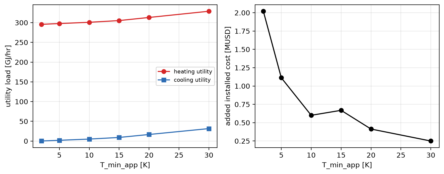
The T_min_app trade-off on the quickstart system. Left: the heating
utility load rises from 2.957e+08 kJ/hr at 2 K to 3.289e+08 kJ/hr at 30 K
and the cooling utility load from 9.219e+04 to 3.157e+07 kJ/hr, so less heat
is recovered as the approach widens. Right: the added installed cost of the
network falls over the same range, from 2.02e+06 USD at 2 K to 2.496e+05
USD at 30 K, most of the drop happening between 2 and 10 K; the bump at
15 K is the best-effort network that needs more exchangers once the pinch
has moved. The default 5 K used throughout this tutorial sits on the steep
part of the cost curve: 2.977e+08 kJ/hr of heating, 1.936e+06 kJ/hr of
cooling and 1.112e+06 USD of added installed cost. Choosing T_min_app is
choosing a point on these two curves; the economically sensible one depends
on utility prices and on the cost of exchanger area, neither of which the
network optimizes for you.#
Scoping the analysis#
By default the network analyzes every unit of the system it belongs to. Two
constructor options change that. units restricts the analysis to a given
set of unit operations – either an iterable of units, or a callable returning
one, which is evaluated at simulation time so that the set may depend on the
converged flowsheet; leaving it as None (the default) means all units of
the system. ignored works the other way round: it names units whose heat
utilities are dropped from the analysis, again as an iterable or a callable.
Whatever survives both filters is collected with
bst.process_tools.heat_exchanger_utilities_from_units, and utilities with a
zero duty are discarded, leaving one process stream per remaining utility.
Excluding a unit is not only an exclusion from the synthesis: it is an
exclusion from the accounting as well. original_heat_util_load and
original_cool_util_load are sums over the utilities that were analyzed, so
the “before” figures move too. Ignoring D1_H1, the cooler on the column’s
bottoms product, makes the point:
HXN.T_min_app = 5.
HXN.ignored = [D1_H1]        # leave the bottoms cooler out of the analysis
sys.simulate()
print(f'streams in the network: {len(HXN.stream_life_cycles)}')
print(f'heating utility: {HXN.original_heat_util_load:.4g} -> {HXN.actual_heat_util_load:.4g} kJ/hr')
print(f'cooling utility: {HXN.original_cool_util_load:.4g} -> {HXN.actual_cool_util_load:.4g} kJ/hr')
HXN.ignored = None
streams in the network: 4
heating utility: 3.609e+08 -> 3.42e+08 kJ/hr
cooling utility: 1.797e+07 -> 0 kJ/hr
Four streams are analyzed instead of the five of Quickstart, and the
one that left carried most of the recoverable heat of this system. On the
cooling side the pool itself shrinks: chapter 1 reported 6.201e+07 ->
1.936e+06 kJ/hr, and here the same two numbers read 1.797e+07 ->
0 kJ/hr. The remaining cooling demand is recovered completely – the process
exchangers bring every remaining hot stream to its outlet, and a stream served
that way passes through its utility exchanger untouched, so no cooling
utility is left at all – but it is a much smaller demand, and the cooling
actually saved falls with it. The
heating side shows the loss directly, since its pool is unchanged: the same
3.609e+08 kJ/hr of heating is only reduced to 3.42e+08 kJ/hr, against
2.977e+08 kJ/hr when D1_H1 was in scope. The bottoms cooler is a large,
high-temperature hot stream, and without it there is far less heat available
to serve the column’s reboiler. Setting ignored back to None restores
the full analysis on the next simulation.
Other options#
The remaining keyword arguments of HeatExchangerNetwork are
listed in the API Reference reference; what each of them does to the
synthesis is described below. Four of them – Qmin, force_ideal_thermo,
avoid_recycle and sort_hus_by_T – are passed straight through to
synthesize_network(), which can also be called directly on a
list of heat utilities.
Qmin is a duty floor, in kJ/hr, defaulting to 1e-3. A planned exchanger
whose duty is below it (Q < Qmin) is dropped from the plan and its duty
left to the utilities, which keeps numerically negligible matches out of the
network; the streams simply carry that heat on to their next match or to their
utility exchangers. Dropping a match never makes another one infeasible, but a
large Qmin can cost MER, and HXN.synthesis_info['qmin_dropped'] lists
what it removed. The same value is passed to the pinch diagram, where a utility
exchanger whose enthalpy change is at or below it (<=, rather than the
strict < of the synthesis) is not marked with a circle – the reason a
stream that finishes on process heat alone carries no utility symbol.
cache_network (default False) reuses a synthesized topology across
simulations, which is worth doing when the same system is simulated many times
with slightly different inputs, as in a Monte Carlo or a sensitivity analysis.
When it is on and a network has already been synthesized, the units owning the
current heat utilities are compared with the exchangers behind the cached one;
if the sets are identical the cached network is kept and only the stream states
and the exchanger specifications are updated. Each life cycle’s first inlet is
copied from the current stream. Each process exchanger keeps, as the enthalpy
limit of the stream its side of the pinch must serve completely (the hot
stream above the pinch, the cold stream below it), the same fraction of that
stream’s duty as at synthesis, so a changed feed rescales every stage instead
of letting the first one take the whole duty; its partner transfers what that
limit sets, but never past its own outlet, and takes the rest to its utility
exchanger, which brings every stream to its new outlet enthalpy. A reused
network is not planned again, so it need not be at MER for the new duties,
and synthesis_info still describes the synthesis that produced it. The
reused network is then re-converged and re-checked stream by stream: the
outlet of each life cycle must reproduce the original exchanger’s outlet in
composition, pressure and enthalpy, and each stream’s original exchanger must
have a finite installed cost. If any of those checks fails, hensmith warns with
a RuntimeWarning saying that the cache algorithm failed and the cached
network was ignored, discards the cache and synthesizes a fresh network. The
energy balance is treated the same way but silently: a cached network whose
energy balance error exceeds the tolerance is discarded and re-synthesized
without a warning, and a warning is issued only if the freshly synthesized
network also fails.
replace_unit_heat_utilities (default False) changes where the savings
are reported. By default the facility carries the difference between the new
and the original utilities as its own heat_utilities, which is why the
utility rows of its results table are negative (Quickstart), and the
original units keep the utilities they had before integration. With the option
on, each synthesized utility exchanger’s heat utility is copied onto the
corresponding original heat utility instead and the owner’s utility cost is
reloaded, so the process units themselves report the reduced duties, and the
facility is left with no heat_utilities of its own. The option applies only
when at least one process exchanger was synthesized; if the synthesis produced
no matches, the facility reports no utilities and no added cost either way.
avoid_recycle (default False) forbids matching the same hot/cold stream
pair more than once anywhere – neither twice on one side of the pinch nor once
on each side. Without it, the planner may match a pair repeatedly: alternating
two partners in series emulates a stream split, and some unsplit MER networks
need it (the repeated exchangers carry a suffix, HX_3_2_cs_2 for the second
one, say). Two exchangers between the same two streams can close a loop in the
network, which its System tears at a recycle stream and converges by
fixed-point iteration. Turning the option on trades those networks – and
possibly MER with them – for a network in which no two exchangers connect the
same pair of streams.
force_ideal_thermo (default False) runs the analysis on copies of the
streams made with ideal thermodynamics (i.thermo.ideal()), and the
synthesized exchangers inherit that property package. It is an escape hatch for
systems whose rigorous VLE is expensive or fragile; the network it produces is
only as accurate as that assumption.
sort_hus_by_T (default False) reorders the streams before the analysis:
heating utilities are sorted by inlet temperature in descending order and
cooling utilities in ascending order. Heating utilities always precede cooling
ones in the rearranged list regardless, and it is that list that fixes the
stream indices used by every per-stream array, by the stream life cycles and by
the pinch diagram. The order does not change the targets; it breaks ties in
the planner’s search, so sorting can change the network that comes out. The
default order is by signed duty, which is how the
facility hands the utilities to the synthesis: cold streams from the smallest
heating duty up, hot streams from the largest cooling duty down.
acceptable_energy_balance_error overrides, for one instance, the class
attribute of the same name. It is a fraction, not a percentage: the default
0.02 means 2 %. After convergence the network’s heat flows are compared
with the original ones, and the absolute deviation from unity of that ratio is
tested against this tolerance; energy_balance_percent_error reports the
same quantity multiplied by 100. Exceeding it warns with a RuntimeWarning,
or raises a RuntimeError if the class attribute
raise_energy_balance_error is set to True.
A larger system#
The quickstart system has five streams and produces four process exchangers.
The system below has ten streams and produces ten, on both sides of the pinch,
which is enough for the structure of a synthesized network to be visible. It is the ten-stream case of
the regression suite, tests/test_hxn_regression.py::case_10_ten_streams,
inlined here rather than imported from tests: five hot streams – two
condensers (H1, H2), one partial condensation (H5) and two liquid
coolers, at two different pressures – and five cold streams, two of which are
taken past their bubble point with rigorous VLE (C2, C3).
bst.settings.set_thermo(['Water', 'Ethanol'], cache=True)
bst.main_flowsheet.set_flowsheet('ten_streams')
units = [utility_hx('H1', 355., 101325., 'g', 320., Ethanol=300.),
         utility_hx('H2', 420., 5e5, 'g', 340., Water=150.),
         utility_hx('H3', 395., 5e5, 'l', 330., Water=1000.),
         utility_hx('H4', 370., 101325., 'l', 310., Ethanol=700.),
         utility_hx('H5', 380., 101325., 'g', 372.5, Water=100.),   # partial condensation
         utility_hx('C1', 300., 101325., 'l', 360., Water=2000.),
         boiling_hx('C2', 330., 101325., 380., Water=200.),
         boiling_hx('C3', 320., 101325., 352., Ethanol=400.),
         utility_hx('C4', 310., 101325., 'l', 345., Water=400., Ethanol=400.),
         utility_hx('C5', 340., 101325., 'l', 390., Water=600.)]
HXN10 = HeatExchangerNetwork('HXN', T_min_app=5.)
sys10 = bst.System.from_units('sys10', units=[*units, HXN10])
sys10.simulate()
hus = HXN10.original_heat_utils
streams_inlet = [hu.unit.ins[0].copy() for hu in hus]
streams_quenched = [hu.unit.outs[0].copy() for hu in hus]
for s in streams_quenched: s.vle(H=s.H, P=s.P)
table = problem_table(streams_inlet, streams_quenched, [hu.duty < 0 for hu in hus], 5.)
print(f'process exchangers: {len(HXN10.new_HXs)}')
print(f'hot utility:  target {table.hot_util_load:.4g}, network {HXN10.actual_heat_util_load:.4g} kJ/hr')
print(f'cold utility: target {table.cold_util_load:.4g}, network {HXN10.actual_cool_util_load:.4g} kJ/hr')
# Those loads are utility-side (duty = unit_duty / heat transfer
# efficiency); the targets are process-side enthalpy differences, so
# sum the process-side duties of the network's utility exchangers too.
new_hus = [hu for hx in HXN10.new_HX_utils for hu in hx.heat_utilities]
heat = sum(hu.unit_duty for hu in new_hus if hu.unit_duty > 0)
cool = -sum(hu.unit_duty for hu in new_hus if hu.unit_duty < 0)
print(f'hot utility,  process side: target {table.hot_util_load:.4g}, network {heat:.4g} kJ/hr')
print(f'cold utility, process side: target {table.cold_util_load:.4g}, network {cool:.4g} kJ/hr')
print(f'energy balance error: {HXN10.energy_balance_percent_error:.2g} %')
print(f"synthesis status: {HXN10.synthesis_info['status']}")
fig, ax = HXN10.plot_pinch_diagram()
process exchangers: 10
hot utility:  target 1.447e+07, network 1.523e+07 kJ/hr
cold utility: target 8.462e+06, network 8.462e+06 kJ/hr
hot utility,  process side: target 1.447e+07, network 1.447e+07 kJ/hr
cold utility, process side: target 8.462e+06, network 8.462e+06 kJ/hr
energy balance error: 2e-12 %
synthesis status: mer
The targets come from problem_table() applied to the same
streams the facility synthesized from, exactly as in Pinch analysis and targets.
The comparison is printed twice because there are two conventions in play. The
facility’s actual_heat_util_load and actual_cool_util_load are
utility-side loads: the duty an agent must supply, which includes that agent’s
heat transfer efficiency. The problem table knows nothing about agents – its
targets are process-side enthalpy differences. Summing the unit_duty of the
new utility exchangers instead, as tests/test_hxn_regression.py does, gives
the process-side loads that are comparable with the targets. On the hot side
the two differ: 1.523e+07 kJ/hr utility-side against 1.447e+07 kJ/hr
process-side, for a target of 1.447e+07 kJ/hr. On the cold side the cooling
agents used here need no such correction and both read 8.462e+06 kJ/hr, against
a target of 8.462e+06 kJ/hr. The network reaches both targets – the synthesis
reports mer – and those process-side numbers, 1.447e+07 and
8.462e+06 kJ/hr, are the values the regression suite records for this case.
Its energy balance error is 2e-12 %.
The phase changes of these streams are what make this case demanding. Two
condensers, a partial condensation and two streams boiled past their bubble
points put flat and steep stretches into the stream curves, and a network
checked only at the terminals of its exchangers could let two streams cross
inside one of them. hensmith keeps T_min_app everywhere inside every
exchanger, on the exact stream states, so its targets and its network hold for
the real streams.
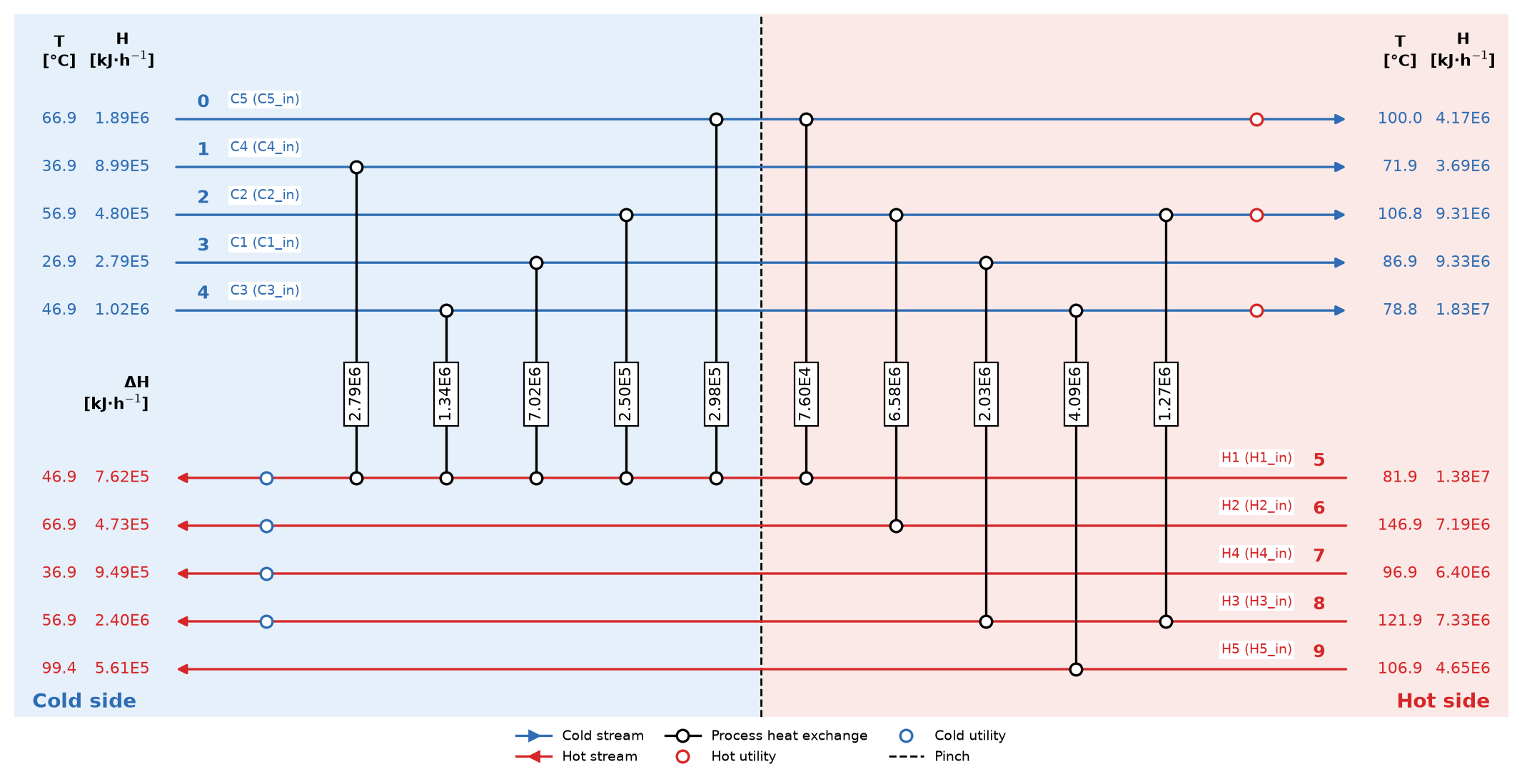
The synthesized ten-stream network. The five cold streams (blue, indices 0
to 4) run left to right and the five hot streams (red, indices 5 to 9) right
to left, each annotated with its inlet and outlet temperature and enthalpy
flow, the outlets being the quenched end states the analysis works from. The
ten vertical connectors are the process exchangers, each labelled with its
duty in kJ/hr; five of them lie to the left of the dashed pinch line, in the
cold-side design, and five to the right, in the hot-side design. Streams 0
(C5) and 5 (H1) are matched with each other on both sides of the
pinch, which closes a loop in the network that its System tears and
converges. Three cold streams still need a hot utility at their outlet (open
red circles on the right) and four hot streams a cold utility (open blue
circles on the left); the others are brought to their outlets by process
heat exchange alone. The shaded background marks the two sides of the pinch.#
Where to next#
Key Concepts – the pinch concepts, the MER planner and the validation behind everything shown in this tutorial.
API Reference – the full API reference, including a table of every constructor option and every attribute the facility sets.