
Anatomy of a synthesized network#
Quickstart reported what the network saved and Pinch analysis and targets
where those targets come from. Neither looked at the network itself. This
chapter opens it: the flowsheet and System the facility builds for its own
exchangers, the naming that makes them readable, the per-stream life cycles
that record which exchangers each stream passes through and in what order, the
per-stream pinch temperatures that split the design into its two sides, the
options of the pinch diagram, and the cost and utility accounting the facility
reports.
Every number and figure below is output of the code shown on this page. The system built here is chapter 1’s build repeated verbatim, so this page runs on its own.
import matplotlib.pyplot as plt
import biosteam as bst
from hensmith import HeatExchangerNetwork

bst.settings.set_thermo(['Water', 'Methanol', 'Glycerol'], cache=True)
bst.main_flowsheet.set_flowsheet('quickstart')
feed1 = bst.Stream('feed1', flow=(8000, 100, 25))
feed2 = bst.Stream('feed2', flow=(10000, 1000, 10))
D1 = bst.ShortcutColumn('D1', ins=feed1,
                        outs=('distillate', 'bottoms_product'),
                        LHK=('Methanol', 'Water'),
                        y_top=0.99, x_bot=0.01, k=2,
                        is_divided=True)
D1_H1 = bst.HXutility('D1_H1', ins=D1.outs[1], T=300)
D1_H2 = bst.HXutility('D1_H2', ins=D1.outs[0], T=300)
F1 = bst.Flash('F1', ins=feed2, outs=('vapor', 'liquid'), V=0.9, P=101325)
HXN = HeatExchangerNetwork('HXN', T_min_app=5.)
sys = bst.System.from_units('sys', units=[D1, D1_H1, D1_H2, F1, HXN])
sys.simulate()
The network flowsheet#
By default, the facility never touches the streams or exchangers of the system
it integrates. Everything it synthesizes – stream copies, process exchangers,
utility exchangers – is created in a flowsheet of its own, and gathered into a
System of its own.
print(HXN.HXN_flowsheet)
print(HXN.HXN_sys)
print([unit.ID for unit in HXN.HXN_sys.units])
sys_HXN
sys_HXN
['HX_0_2_hs', 'HX_1_2_hs', 'HX_1_4_hs', 'HX_1_3_hs', 'Util_2_cs', 'Util_3_cs', 'Util_4_cs', 'Util_0_hs', 'Util_1_hs']
HXN.HXN_flowsheet is that flowsheet, a bst.Flowsheet named after the
system it belongs to, sys.ID + '_HXN' – here sys_HXN. It is created
each time the facility synthesizes a network, and its registries are cleared
before synthesis, so the network’s IDs neither collide with the original
flowsheet’s nor accumulate across repeated simulations.
HXN.HXN_sys is the bst.System built from the synthesized units. It is
named after the flowsheet, sys_HXN, in whose system registry it is
registered – so HXN.HXN_flowsheet.system.sys_HXN resolves to it, just as
the exchangers resolve through HXN.HXN_flowsheet.unit. It is an ordinary
System holding the nine units listed on the third line. They are listed in
the order the system simulates them, which follows the streams: after
synthesis every stream’s stages are rewired in series, each stage feeding the
next, and the path is a topological order of those connections, ties broken
by the order in which the synthesis returned the exchangers – the process
exchangers in plan order, then the utility exchangers, hot streams first.
HX_0_2_hs therefore runs first: it is the first stage of both of its
streams, while HX_1_2_hs has to wait for stream 2 to leave it. Where the
stages of a network form a loop – a pair of streams matched on both sides of
the pinch, or two streams matched repeatedly in alternation – the loop is
torn at a recycle stream and converged by the system’s own fixed-point
solver.
The IDs carry the whole topology. A process exchanger is an HXprocess named
HX_<cold>_<hot>_hs when it lies above the pinch, in the hot-side design, and
HX_<hot>_<cold>_cs when it lies below the pinch, in the cold-side design –
note that the two orders differ: a cold-side exchanger names its hot stream
first, a hot-side one its cold stream first, and in both the first number is
the stream at port 0. When the same two streams are matched more than once on
the same side, the second and later exchangers carry a suffix, _2,
_3, …, in the order the hot stream meets them (HX_3_2_cs_2, say). A
utility exchanger is an HXutility named Util_<index>_hs for a cold
stream, which is finished by a hot utility above the pinch, and
Util_<index>_cs for a hot stream, which is finished by a cold utility below
it. The indices are stream indices: positions in the rearranged utility list of
synthesize_network(), cold streams first and then hot ones, as
described in Pinch analysis and targets. The stream copies are named after the
exchanger they touch, s_<index>__<exchanger> on the way in and
<exchanger>__s_<index> on the way out.
All four process exchangers of this network end in _hs: every match lies
above the pinch, which is the same fact as the pinch diagram of
Quickstart showing all four connectors to the right of the pinch
line. Below the pinch there is nothing to design: no cold stream needs heat
there (stream 1 enters exactly at the pinch temperature and stream 0 above
it, as the pinch temperatures below show), so the only stream below it, hot
stream 2, is finished by its cooler.
HXN.HXN_sys.diagram()
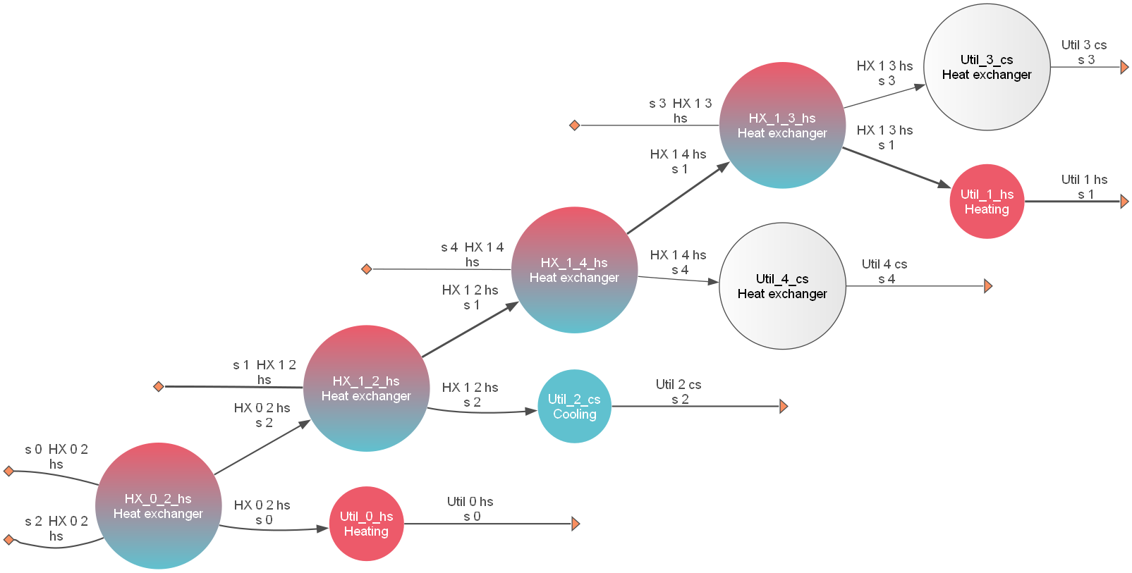
The synthesized network as its own flowsheet, sys_HXN. The four
two-inlet nodes are the process exchangers; each takes one cold and one hot
stream copy and passes both on. The five single-inlet nodes are the utility
exchangers that finish each stream: Util_0_hs and Util_1_hs are
heating, Util_2_cs is cooling, and Util_3_cs and Util_4_cs are
drawn grey because they carry no utility at all – their inlet and outlet
enthalpies are equal, 2.47e+06 and 7.18e+05 kJ/hr, so streams 3 and 4 are
brought to their outlet states by process heat exchange alone. The stream
names show the wiring: s_1__HX_1_2_hs enters HX_1_2_hs carrying
stream 1, and HX_1_2_hs__s_1 leaves it and enters HX_1_4_hs.#
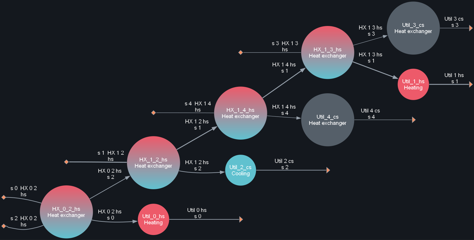
The synthesized network as its own flowsheet, sys_HXN. The four
two-inlet nodes are the process exchangers; each takes one cold and one hot
stream copy and passes both on. The five single-inlet nodes are the utility
exchangers that finish each stream: Util_0_hs and Util_1_hs are
heating, Util_2_cs is cooling, and Util_3_cs and Util_4_cs are
drawn grey because they carry no utility at all – their inlet and outlet
enthalpies are equal, 2.47e+06 and 7.18e+05 kJ/hr, so streams 3 and 4 are
brought to their outlet states by process heat exchange alone. The stream
names show the wiring: s_1__HX_1_2_hs enters HX_1_2_hs carrying
stream 1, and HX_1_2_hs__s_1 leaves it and enters HX_1_4_hs.#
Stream life cycles#
A flowsheet of nine units says what exists; it does not say, for one stream,
what happens to it. That is what a StreamLifeCycle records.
The facility builds one per stream after synthesis, aligned with
HXN.original_heat_exchangers, and stores them in
HXN.stream_life_cycles.
for life_cycle in HXN.stream_life_cycles:
    life_cycle.show()
StreamLifeCycle: Stream_0, cold
	life_cycle:
		<LifeStage: <HXprocess: HX_0_2_hs>, H_in = 5.38e+06 kJ/hr, H_out = 4.24e+07 kJ/hr>
		<LifeStage: <HXutility: Util_0_hs>, H_in = 4.24e+07 kJ/hr, H_out = 6.92e+07 kJ/hr>

StreamLifeCycle: Stream_1, cold
	life_cycle:
		<LifeStage: <HXprocess: HX_1_2_hs>, H_in = 0 kJ/hr, H_out = 5.05e+06 kJ/hr>
		<LifeStage: <HXprocess: HX_1_4_hs>, H_in = 5.05e+06 kJ/hr, H_out = 5.08e+06 kJ/hr>
		<LifeStage: <HXprocess: HX_1_3_hs>, H_in = 5.08e+06 kJ/hr, H_out = 2.3e+07 kJ/hr>
		<LifeStage: <HXutility: Util_1_hs>, H_in = 2.3e+07 kJ/hr, H_out = 2.79e+08 kJ/hr>

StreamLifeCycle: Stream_2, hot
	life_cycle:
		<LifeStage: <HXprocess: HX_0_2_hs>, H_in = 4.52e+07 kJ/hr, H_out = 8.12e+06 kJ/hr>
		<LifeStage: <HXprocess: HX_1_2_hs>, H_in = 8.12e+06 kJ/hr, H_out = 3.07e+06 kJ/hr>
		<LifeStage: <HXutility: Util_2_cs>, H_in = 3.07e+06 kJ/hr, H_out = 1.14e+06 kJ/hr>

StreamLifeCycle: Stream_3, hot
	life_cycle:
		<LifeStage: <HXprocess: HX_1_3_hs>, H_in = 2.04e+07 kJ/hr, H_out = 2.47e+06 kJ/hr>
		<LifeStage: <HXutility: Util_3_cs>, H_in = 2.47e+06 kJ/hr, H_out = 2.47e+06 kJ/hr>

StreamLifeCycle: Stream_4, hot
	life_cycle:
		<LifeStage: <HXprocess: HX_1_4_hs>, H_in = 7.51e+05 kJ/hr, H_out = 7.18e+05 kJ/hr>
		<LifeStage: <HXutility: Util_4_cs>, H_in = 7.18e+05 kJ/hr, H_out = 7.18e+05 kJ/hr>
A life cycle has the attributes index, the stream’s index; name,
s_<index>; cold, True for a heated stream and False for a cooled
one; and life_cycle, the list of stages. It is recovered from IDs alone:
each exchanger ID is parsed – HX_<a>_<b>_<hs|cs>, with an optional
_<n> suffix, or Util_<a>_<hs|cs> – the first number being the stream
at port 0 and the second the stream at port 1, so a stream index is matched
exactly and never as a substring of another index. The stages are then sorted
by inlet enthalpy, ascending for a cold stream and descending for a hot one,
which is flow direction in both cases since a cold stream gains enthalpy as it
goes and a hot stream loses it (ties, which only stages without duty can
produce, put the stream’s first side of the pinch first and its utility
last).
Read stream 1, the longest life cycle here: it passes HX_1_2_hs,
HX_1_4_hs and HX_1_3_hs and then its utility exchanger Util_1_hs,
its enthalpy rising 0, 5.05e+06, 5.08e+06, 2.3e+07 and finally 2.79e+08 kJ/hr.
Its first exchanger is the match the pinch design method asks for: stream 1
enters exactly at the pinch temperature, and HX_1_2_hs pairs it there with
stream 2, the only hot stream that reaches the pinch, from which the planner
builds the hot-side design outward. Stream 2 runs the other way, 4.52e+07 to
8.12e+06 to 3.07e+06 kJ/hr through two process exchangers and then to
1.14e+06 kJ/hr through Util_2_cs. Each
stage’s outlet enthalpy is the next stage’s inlet enthalpy because the facility
rewires the units after synthesis, making each stage’s outlet stream the inlet
of the following stage. Streams 3 and 4 end on a stage whose inlet and outlet
enthalpies are equal, 2.47e+06 and 7.18e+05 kJ/hr: their utility exchangers
have nothing left to do.
One stage on its own:
stage = HXN.stream_life_cycles[1].life_cycle[0]
print(stage.unit, '| stream position', stage.index)
print(stage.s_in.ID, '->', stage.s_out.ID)
print(f'{stage.H_in:.4g} -> {stage.H_out:.4g} kJ/hr')
HX_1_2_hs | stream position 0
s_1__HX_1_2_hs -> HX_1_2_hs__s_1
0 -> 5.051e+06 kJ/hr
A LifeStage holds only two things, unit and index; everything else
is a property read from the unit when accessed. index is the position of
this stream in the exchanger’s ins and outs – 0 or 1 for an
HXprocess, always 0 for an HXutility. Here it is 0, because a hot-side
process exchanger is constructed with its cold stream first. s_in and
s_out are unit.ins[index] and unit.outs[index], and H_in and
H_out are their enthalpies, so a life cycle always reflects the current
state of the network rather than a snapshot taken at synthesis. This stage
takes stream 1 from 0 to 5.051e+06 kJ/hr.
Per-stream pinch temperatures#
The pinch analysis produces three arrays indexed like the life cycles, which
the facility stores as HXN.inlet_Ts, HXN.outlet_Ts and
HXN.pinch_Ts. The first two are each stream’s inlet temperature and its
quenched outlet temperature (Pinch analysis and targets). The third is the
temperature at which a stream crosses the process pinch on its own scale,
where it passes from the cold-side design into the hot-side design. It is
reported for information: the synthesizer cuts every stream at the pinch on
the stream’s temperature-enthalpy curve itself, and pinch_Ts summarizes
where that cut lies.
for i, life_cycle in enumerate(HXN.stream_life_cycles):
    kind = 'cold' if life_cycle.cold else 'hot '
    print(f'stream {i} ({kind}): in {HXN.inlet_Ts[i] - 273.15:5.1f} °C, '
          f'pinch {HXN.pinch_Ts[i] - 273.15:5.1f} °C, out {HXN.outlet_Ts[i] - 273.15:5.1f} °C')
stream 0 (cold): in  33.2 °C, pinch  33.2 °C, out  99.5 °C
stream 1 (cold): in  25.0 °C, pinch  25.0 °C, out  95.9 °C
stream 2 (hot ): in  98.2 °C, pinch  30.0 °C, out  26.8 °C
stream 3 (hot ): in  65.4 °C, pinch  64.9 °C, out  64.9 °C
stream 4 (hot ): in  64.9 °C, pinch  64.8 °C, out  64.8 °C
The process pinch of this system is a single shifted temperature, 298.15 K
(Pinch analysis and targets), which stands for two real ones: 25.0 °C for cold
streams and, T_min_app higher, 30.0 °C for hot streams. Each stream is then
classified against the pinch temperature of its own kind.
A stream that reaches the pinch is cut there, and its
pinch_Tis the pinch temperature of its kind. Stream 2 crosses it, 98.2 to 26.8 °C, and stream 1 enters exactly at it, 25.0 °C; they are cut at 30.0 and 25.0 °C respectively.A stream whose outlet stops short of the pinch never reaches it, and its
pinch_Tis its own outlet temperature: it lies wholly on one side, and the cut is a formality at its far end. Streams 3 and 4 are hot streams that cool only to 64.9 and 64.8 °C, far above the 30.0 °C hot-stream pinch, and those outlet temperatures are exactly whatpinch_Tsreports for them.A stream whose inlet is already past the pinch is likewise not cut, and its
pinch_Tis its inlet temperature. Stream 0 is a cold stream entering at 33.2 °C, above the 25.0 °C cold-stream pinch, so itspinch_Tis 33.2 °C.
That last clause also catches isothermal and non-monotone streams – a stream
whose outlet lies on the wrong side of its inlet for the sign of its duty, such
as a cold stream whose equilibrium outlet ends up cooler than it entered.
These get pinch_T = T_in too, but only as a label. The synthesis treats
them as the problem table does, as a point load: their whole duty sits at their
outlet temperature, on whichever side of the pinch that temperature lies (and,
exactly at the pinch, on the side the problem table’s cascade assigns the
point loads there), and such a stream enters its first process exchanger in
the equilibrium state at its inlet enthalpy.
Reading the pinch diagram#
plot_pinch_diagram() draws the life cycles above. Called as
HXN.plot_pinch_diagram, the facility supplies the life cycles, the inlet
and outlet temperatures, the hot-side and cold-side exchanger lists, its
Qmin and the original exchangers, and forwards file and every other
keyword argument. Those remaining arguments are:
show_units,show_auxiliary_unitsandshow_stream_IDsThe three parts of each stream’s label, built from its original heat exchanger and joined as
<unit> - <auxiliary> (<inlet stream ID>): respectively the ID of the unit owning that exchanger, the name of the exchanger within its owner when it is an auxiliary one (condenserand the like), and the ID of that exchanger’s inlet stream. All three default toTrue; with all three off no label is drawn and the original exchangers are not needed, while turning any of them on without those exchangers raisesValueError.show_legendAdds a legend of the six symbols – cold stream, hot stream, process heat exchange, hot utility, cold utility, pinch – below the axes.
axDraws into a
matplotlibaxes provided by the caller instead of creating a figure; the figure returned is then the one that axes belongs to.fileanddpiSave the figure to a path, at the given resolution.
Turning off the labels and the legend leaves the quantitative skeleton of the diagram:
fig, ax = plt.subplots(figsize=(9, 4.4))
HXN.plot_pinch_diagram(show_units=False, show_auxiliary_units=False,
                       show_stream_IDs=False, show_legend=False, ax=ax)
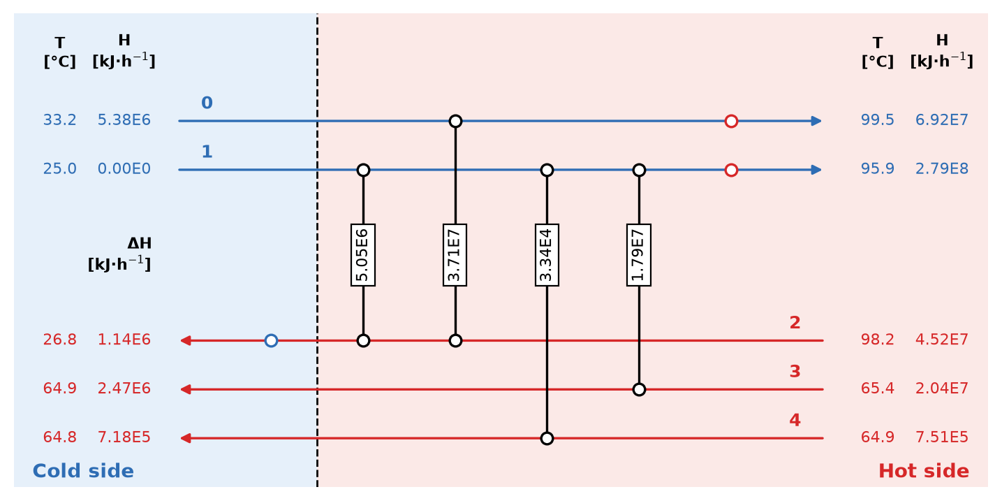
The same network as the pinch diagram of Quickstart, with
show_stream_IDs=False and show_legend=False – and the two unit-label
options off as well – drawn into an axes created by the caller. Only the
stream annotations and the legend are gone: the T and H columns on
both sides remain, and so do the boxed exchanger duties in the ΔH row,
the bold stream index at the inlet of each stream, the dashed pinch line and
the Cold side and Hot side captions. The columns read off the life
cycles above: stream 1 enters at 25.0 °C with 0.00E0 kJ/hr and leaves at
95.9 °C with 2.79E8 kJ/hr, and the first connector it meets carries the
5.05E6 kJ/hr of its first stage. The four duties are the same four as in
Quickstart.#
Exchanger columns are ordered independently on each side of the pinch, by
_order_exchanger_columns. Every stream’s stage order is a chain of
precedence constraints between the exchangers it meets – reversed for hot
streams, which are drawn right to left – and a topological sort of that graph
(Kahn’s algorithm, ties broken by the order in which the synthesis returned the
exchangers, the plan order from the pinch outward) lays them out so that every
stream meets its exchangers in flow direction. That is why stream 1 reads its
three connectors left to right in exactly the order of its life cycle.
Constraints that contradict each other, which would require some stream to
flow backwards, cannot be satisfied by any ordering; the given order is then
used unchanged.
Energy balance and cost accounting#
What the facility reports about itself is one consistency check and a set of differences.
print(f'energy balance error: {HXN.energy_balance_percent_error:.2g} % '
      f'(warns above {100 * HXN.acceptable_energy_balance_error:.0f} %)')
print(f'original exchangers, purchase cost: {sum(HXN.original_purchase_costs):.4g} USD')
print(f'new process exchangers, purchase:   {sum(HXN.new_purchase_costs_HXp):.4g} USD')
print(f'new utility exchangers, purchase:   {sum(HXN.new_purchase_costs_HXu):.4g} USD')
print(f'facility purchase cost (added):     {HXN.purchase_costs["Heat exchangers"]:.4g} USD')
print(f'facility installed cost (added):    {HXN.installed_costs["Heat exchangers"]:.4g} USD')
print('facility heat utilities (new minus original):')
for hu in HXN.heat_utilities:
    print(f'  {hu.ID:<20} duty {hu.duty:>11.4g} kJ/hr   cost {hu.cost:>8.4g} USD/hr')
energy balance error: -1.8e-11 % (warns above 2 %)
original exchangers, purchase cost: 3.365e+05 USD
new process exchangers, purchase:   4.734e+05 USD
new utility exchangers, purchase:   2.095e+05 USD
facility purchase cost (added):     3.464e+05 USD
facility installed cost (added):    1.112e+06 USD
facility heat utilities (new minus original):
  low_pressure_steam   duty  -6.324e+07 kJ/hr   cost   -388.8 USD/hr
  chilled_water        duty   4.214e+07 kJ/hr   cost   -210.7 USD/hr
  cooling_water        duty   1.794e+07 kJ/hr   cost   -5.976 USD/hr
energy_balance_percent_error compares the heat the synthesized network
moves with the heat the original exchangers moved. The numerator is twice the
absolute duty of every new process exchanger – twice, because each process
match takes that heat off one stream and puts it onto another – plus the
process-side duty of the new utility exchangers, each agent’s duty
multiplied by its heat_transfer_efficiency. The denominator is the same
product summed over the original utilities. The ratio less one, times 100, is
the reported percentage: -1.8e-11 % here, which is round-off.
The tolerance it is checked against, acceptable_energy_balance_error, is a
fraction, not a percentage: the class attribute is 0.02, that is 2 %, and
the constructor argument of the same name defaults to None, meaning that
the class value is kept. The check is on the absolute error. Exceeding it warns
with a RuntimeWarning naming the error and the tolerance, or raises a
RuntimeError instead if the class attribute raise_energy_balance_error
is set to True.
The costs are differences, clipped at zero. original_purchase_costs is the
purchase cost of each original exchanger, one entry per stream, 3.365e+05 USD
in total here; new_purchase_costs_HXp and new_purchase_costs_HXu are
the same for the synthesized process and utility exchangers, 4.734e+05 and
2.095e+05 USD. The facility’s own purchase_costs['Heat exchangers'] – and
its identical baseline_purchase_costs entry – is max(0, new - original)
over those three sums, 4.734e+05 + 2.095e+05 - 3.365e+05 = 3.464e+05 USD. Its
installed_costs['Heat exchangers'] is formed exactly the same way from the
installed costs of the same exchangers rather than their purchase costs, and
is the larger figure here, 1.112e+06 USD. Clipping at zero means a network
whose exchangers happen to be cheaper than the ones they replace is reported as
adding nothing rather than as a capital credit; and if the synthesis produced
no process exchangers at all, both entries are set to zero and the facility
reports no utilities either.
The utilities are differences too. original_utility_costs holds the
original heat utilities summed by agent – reversed in sign, since they are the
very objects that were negated to form the difference – and
new_utility_costs holds the new utility exchangers’ utilities summed by
agent. HXN.heat_utilities is the sum of the two, that is new - original,
which is why every cost printed above is negative: -388.8 USD/hr of low
pressure steam, -210.7 USD/hr of chilled water and -5.976 USD/hr of cooling
water are savings. The duties carry the sign convention of their agent, so the
steam duty is negative, -6.324e+07 kJ/hr, while the chilled and cooling water
duties are positive, 4.214e+07 and 1.794e+07 kJ/hr, because cooling duties are
negative to begin with and a positive difference again means less of them.
Setting replace_unit_heat_utilities=True moves this reporting onto the
process units instead, as Configuring the network and a larger system describes.
Where to next#
Configuring the network and a larger system – the constructor options of the facility, what
T_min_appandignoredchange, and a ten-stream network.Key Concepts – the pinch concepts, the MER planner, and what a synthesized network is and is not guaranteed to be.
API Reference – the full API reference.