
Pinch analysis and targets#
The utility targets behind Quickstart are not fitted numbers: they
come from a temperature-interval heat cascade – the problem table – built on
exactly the streams the network is synthesized from. This chapter follows that
computation end to end: how hensmith turns the heat utilities of a simulated
system into hot and cold process streams, what problem_table()
does with them, how the resulting ProblemTable can be
redrawn as composite curves and as a grand composite curve, and how the network
synthesized in chapter 1 compares with the targets those curves define.
Every number and figure below is output of the code shown on this page. The system built here is chapter 1’s build repeated verbatim, so this page runs on its own.
Streams as heat utilities#
import numpy as np
import matplotlib.pyplot as plt
import biosteam as bst
from hensmith import HeatExchangerNetwork
from hensmith.hxn_synthesis import problem_table
A pinch analysis needs process streams, but what a simulated biosteam system
carries is heat utilities: one HeatUtility per heat exchanger, each with a
duty and a reference to the exchanger that owns it. hensmith collects them with
bst.process_tools.heat_exchanger_utilities_from_units over the units in
scope and keeps the ones with a nonzero duty, minus any belonging to units
passed as ignored. Every heating or cooling requirement in the system –
including the auxiliary exchangers inside columns and flashes – therefore
becomes exactly one process stream, and the list of those utilities is kept on
the facility as HXN.original_heat_utils. That attribute holds the list in
the order the synthesizer rearranges it into – every heating utility first,
then every cooling one – so a utility’s position in it is the stream index
used throughout the network and its stream life cycle.
Each utility becomes a pair of end states – an inlet and a quenched outlet –
of one process stream. The inlet is the exchanger’s own inlet,
hu.unit.ins[0]; the outlet is the exchanger’s outlet quenched to
equilibrium at its own enthalpy, s.vle(H=s.H, P=s.P), so that the end state
the analysis works from is an equilibrium state and the enthalpy path between
the two end temperatures is thermodynamically consistent – which matters for
the phase-changing streams that dominate this system. The sign of the duty says
which kind of stream it is: duty > 0 means the exchanger heats its stream,
which is a cold stream in pinch terms, and duty < 0 means it cools it, a
hot stream. That distinction is the is_hot argument of
problem_table(), and this is the same construction the facility
performs internally before synthesis, and that tests/test_hxn_regression.py
uses to compute its reference targets.
The problem table#
The smallest instructive case is a two-stream threshold problem, the example
in the problem_table() docstring: a stream of water is cooled
while a slightly smaller stream of water is heated over an overlapping
temperature range.
bst.settings.set_thermo(['Water'])
hot_in = bst.Stream(Water=1000., T=400., P=5e5, phase='l', units='kmol/hr')
hot_out = hot_in.copy(); hot_out.vle(T=300., P=5e5)
cold_in = bst.Stream(Water=900., T=300., P=5e5, phase='l', units='kmol/hr')
cold_out = cold_in.copy(); cold_out.vle(T=390., P=5e5)
table = problem_table([hot_in, cold_in], [hot_out, cold_out], [True, False], 5.)
print('shifted grid Ts [K]:', table.Ts.size, 'points,', table.Ts[0], 'down to', table.Ts[-1])
print('hot utility target [kJ/hr]: ', round(table.hot_util_load, 3))
print('cold utility target [kJ/hr]:', round(table.cold_util_load, -1))
print('pinch (shifted) [K]:', table.pinch_T)
shifted grid Ts [K]: 25 points, 395.0 down to 295.0
hot utility target [kJ/hr]:  0.0
cold utility target [kJ/hr]: 1445550.0
pinch (shifted) [K]: 395.0
Hot streams are shifted down by T_min_app and cold streams are left
alone. On that shifted scale, two streams at equal temperature are in reality
exactly T_min_app apart, so heat may be cascaded from any shifted
temperature to any lower one without ever violating the minimum approach. The
grid above runs from 395 K, the hot stream’s inlet shifted down by the 5 K
approach, to 295 K, its shifted outlet; the cold stream’s ends, unshifted at
390 and 300 K, lie in between. The grid holds 25 points rather than those four
because it is the union, sorted descending, of the breakpoints of every
stream’s temperature-enthalpy curve. hensmith describes each stream by such a
curve, built once from a handful of flashes: its breakpoints are the stream’s
end temperatures, every phase boundary inside its range, and – since the heat
capacity of liquid water varies with temperature – interior points that keep
a straight line between neighbours within 0.002 K of the true curve. Every
temperature at which a curve bends is therefore a grid point, and nothing that
happens inside an interval can hide a pinch.
Between consecutive grid temperatures, each stream contributes the enthalpy its curve releases or absorbs over that interval, evaluated at its real temperature and clipped to its own enthalpy range, with a positive sign for hot streams and a negative one for cold. Because the grid always contains every breakpoint of a stream’s curve, its own end temperatures among them, those contributions telescope exactly to the stream’s duty: no heat is created or lost by the discretization. Heat that a curve gives up or takes at a single temperature is not spread over an interval at all but enters as a point load at that grid temperature: the latent heat of a pure component boiling or condensing at its saturation temperature, and the whole duty of a stream with no temperature span of its own – an isothermal condenser, or a stream whose outlet moves against its duty, such as a reboiler outlet at equilibrium – which sits at its shifted outlet temperature.
Cascading those contributions down the grid, with no hot utility supplied,
gives the heat leaving each boundary, the residual field. Feasibility
must hold for the heat arriving at each boundary too – the residual before
that boundary’s point loads are applied – because a point source sitting at a
grid temperature cannot serve a sink above it. The worst deficit over both
flows is the minimum hot utility, and its location is the pinch. Here the
cascade never goes negative, which is what a threshold problem means:
hot_util_load is 0.0, all of the surplus leaves as 1445550.0 kJ/hr of cold
utility, and pinch_T reports the top of the grid, 395.0 K.
The quickstart system is the same computation on five streams:
import biosteam as bst
from hensmith import HeatExchangerNetwork

bst.settings.set_thermo(['Water', 'Methanol', 'Glycerol'], cache=True)
bst.main_flowsheet.set_flowsheet('quickstart')
feed1 = bst.Stream('feed1', flow=(8000, 100, 25))
feed2 = bst.Stream('feed2', flow=(10000, 1000, 10))
D1 = bst.ShortcutColumn('D1', ins=feed1,
                        outs=('distillate', 'bottoms_product'),
                        LHK=('Methanol', 'Water'),
                        y_top=0.99, x_bot=0.01, k=2,
                        is_divided=True)
D1_H1 = bst.HXutility('D1_H1', ins=D1.outs[1], T=300)
D1_H2 = bst.HXutility('D1_H2', ins=D1.outs[0], T=300)
F1 = bst.Flash('F1', ins=feed2, outs=('vapor', 'liquid'), V=0.9, P=101325)
HXN = HeatExchangerNetwork('HXN', T_min_app=5.)
sys = bst.System.from_units('sys', units=[D1, D1_H1, D1_H2, F1, HXN])
sys.simulate()
hus = HXN.original_heat_utils
streams_inlet = [hu.unit.ins[0].copy() for hu in hus]
streams_quenched = [hu.unit.outs[0].copy() for hu in hus]
for s in streams_quenched: s.vle(H=s.H, P=s.P)
is_hot = [hu.duty < 0 for hu in hus]
table = problem_table(streams_inlet, streams_quenched, is_hot, T_min_app=5.)
print(f'shifted grid Ts:     {table.Ts.size} points, {table.Ts[0]:.2f} down to {table.Ts[-1]:.2f} K')
print(f'point loads:         {np.count_nonzero(table.point_H)}')
print(f'hot utility target:  {table.hot_util_load:.4g} kJ/hr')
print(f'cold utility target: {table.cold_util_load:.4g} kJ/hr')
print(f'pinch (shifted):     {table.pinch_T:.2f} K')
shifted grid Ts:     175 points, 372.60 down to 295.00 K
point loads:         0
hot utility target:  2.828e+08 kJ/hr
cold utility target: 1.936e+06 kJ/hr
pinch (shifted):     298.15 K
The five streams produce a grid of 175 shifted temperatures, from 372.60 K
down to 295.00 K. Their shifted end temperatures are among them; most of the
rest trace two-phase glides. Every stream here is a mixture of water, methanol
and glycerol, so none boils or condenses at a single temperature: the
column’s reboiler and the flash’s feed heater heat a liquid past its bubble
point and on along a glide, the condenser and the distillate cooler D1_H2
glide from end to end, and the bottoms cooler D1_H1 cools a liquid whose
heat capacity varies with temperature. Each glide and each curved stretch is
sampled until a straight line between neighbouring points is within 0.002 K
of the true curve. With no flat segment in any curve, and every outlet moving
in the direction of its stream’s duty, the table has no point loads at all –
the second line. The condenser is still the most conspicuous stream: it gives
up its latent heat over about half a Kelvin, from 65.4 to 64.9 °C on the real
scale (Anatomy of a synthesized network lists every stream’s end temperatures), and
the distillate cooler takes the stream on from there. The
targets are 2.828e+08 kJ/hr of hot utility and 1.936e+06 kJ/hr of cold utility,
and the pinch is at 298.15 K on the shifted scale. Since hot streams were
shifted down by the 5 K approach, that one shifted temperature stands for two
real ones: 25 °C for the cold streams and 30 °C for the hot ones. It is the
temperature that splits the synthesized network into its hot-side and cold-side
designs, and the dashed line drawn on the pinch diagram of chapter 1.
Composite curves#
hensmith itself ships one plot, the pinch diagram of a synthesized network. The
two curves below are not library functions: they are computed in this
tutorial’s script from the fields of the ProblemTable, and
they are shown here because they are the standard way to read what the table
says before any network exists.
def composite_curves(table, T_min_app):
    """Hot and cold composite curves (real T [K] vs H [kJ/hr]) of a
    ProblemTable. Walking the shifted grid from the coldest boundary up,
    each interval adds the heat of the streams of that kind in it (a
    diagonal segment) and each point load adds heat at constant temperature
    (a horizontal step). Hot streams were shifted down by T_min_app, so
    their real temperature is Ts + T_min_app. The cold curve starts at
    H = cold utility so the curves overlap by exactly the recovered heat
    and the right-hand overhang is the hot utility."""
    Ts = table.Ts
    n = Ts.size
    is_hot = (table.interval_H.sum(axis=1) + table.point_H.sum(axis=1)) > 0

    def build(rows, T_offset, H0):
        interval = np.abs(table.interval_H[rows].sum(axis=0))   # n - 1 intervals
        point = np.abs(table.point_H[rows].sum(axis=0))         # n boundaries
        T, H = [Ts[n - 1] + T_offset], [H0]
        for k in range(n - 1, -1, -1):
            if point[k] > 0:
                T.append(Ts[k] + T_offset); H.append(H[-1] + point[k])
            if k > 0:
                T.append(Ts[k - 1] + T_offset); H.append(H[-1] + interval[k - 1])
        T, H = np.array(T), np.array(H)
        nz = np.flatnonzero(np.diff(H) > 0)   # drop end segments with no stream of this kind
        return T[nz[0]:nz[-1] + 2], H[nz[0]:nz[-1] + 2]

    hot_T, hot_H = build(is_hot, T_min_app, 0.)
    cold_T, cold_H = build(~is_hot, 0., table.cold_util_load)
    return hot_T, hot_H, cold_T, cold_H
Walking the shifted grid upwards from its coldest boundary, each interval adds
the heat of the streams of one kind in it as a diagonal segment, and each point
load adds heat at constant temperature as a horizontal step. The hot curve is
drawn back on the real scale by adding T_min_app to the shifted grid, so
that the vertical distance between the two curves is a real temperature
difference and is nowhere smaller than the approach. The hot curve starts at
H = 0 and the cold curve starts at H equal to the cold utility target,
which places the two so that their horizontal overlap is exactly the heat that
can be recovered and each overhang is exactly one utility target. Ends of the
grid where no stream of that kind exists carry no load, and are trimmed off
rather than drawn as vertical segments.
hot_T, hot_H, cold_T, cold_H = composite_curves(table, T_min_app=5.)
GJ = 1e6  # kJ/hr -> GJ/hr
fig, ax = plt.subplots(figsize=(7.5, 4.2))
ax.axvspan(cold_H[0] / GJ, hot_H[-1] / GJ, color='0.92', lw=0, zorder=0, label='heat recovered')
ax.plot(hot_H / GJ, hot_T - 273.15, color='#d62728', lw=2, label='hot composite')
ax.plot(cold_H / GJ, cold_T - 273.15, color='#2e6db4', lw=2, label='cold composite')
y_lo, y_hi = hot_T[0] - 273.15, cold_T[-1] - 273.15
ax.margins(y=0.12)   # headroom so the utility labels sit inside the frame
# the cold-utility span is ~6 px wide on this axis, too narrow for an arrow:
# bound it with two ticks and label it with a leader
ax.vlines([0, cold_H[0] / GJ], y_lo - 1.5, y_lo + 1.5, color='k', lw=0.8, zorder=3)
ax.annotate(f'cold utility {table.cold_util_load:.3g} kJ/hr', xy=(cold_H[0] / 2 / GJ, y_lo),
            xytext=(30, -18), textcoords='offset points', fontsize=8,
            arrowprops=dict(arrowstyle='-', lw=0.6, shrinkB=4))
ax.annotate('', xy=(hot_H[-1] / GJ, y_hi), xytext=(cold_H[-1] / GJ, y_hi), arrowprops=dict(arrowstyle='<->'))
ax.text((hot_H[-1] + cold_H[-1]) / 2 / GJ, y_hi + 2, f'hot utility {table.hot_util_load:.3g} kJ/hr',
        ha='center', va='bottom', fontsize=8)
ax.set_xlabel('H [GJ/hr]'); ax.set_ylabel('T [°C]')
ax.legend(loc='lower right', fontsize=8); ax.grid(alpha=0.3)
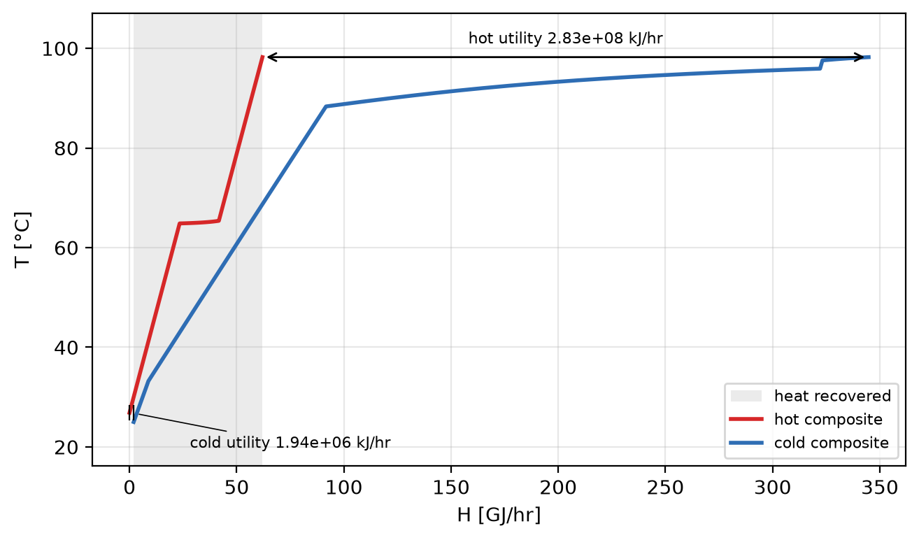
Composite curves of the quickstart system. The hot composite (red) begins at
H = 0 at its cold end and ends where the last hot stream is exhausted;
its near-horizontal step is the column condenser condensing over about half
a Kelvin, from 65.4 to 64.9 °C. The cold composite (blue) begins at the cold
utility target, 1.936e+06 kJ/hr, and ends at that offset plus the total
heating demand of the system. The shaded band where the two overlap
horizontally is the heat that process-to-process exchange can recover; the
overhang to the left of it is the cold utility target, 1.936e+06 kJ/hr, and
the overhang to the right is the hot utility target, 2.828e+08 kJ/hr, both
annotated on the figure to three significant figures. The
cold composite extends far to the right of the hot one because this system
needs a great deal more heating than it has cooling available.#
The same cascade can also be plotted directly, as a grand composite curve:
def grand_composite(table):
    """Heat cascaded through each shifted grid temperature when the minimum
    hot utility is supplied: the value arriving at each boundary and the
    value leaving it after its point loads (a horizontal step where a
    stream is isothermal). It touches zero at the pinch."""
    leaving = table.residual + table.hot_util_load
    arriving = leaving - table.point_H.sum(axis=0)
    H = np.column_stack([arriving, leaving]).ravel()
    T = np.repeat(table.Ts, 2)
    return H, T
H_cascade, T_cascade = grand_composite(table)
fig, ax = plt.subplots(figsize=(5, 4.2))
ax.plot(H_cascade / GJ, T_cascade - 273.15, color='k', lw=2)
ax.axvline(0, color='k', lw=0.8, ls='--')
ax.plot([0], [table.pinch_T - 273.15], 'o', mfc='w', mec='k', ms=8)
ax.annotate(f'pinch  {table.pinch_T - 273.15:.1f} °C (shifted)', xy=(0, table.pinch_T - 273.15),
            xytext=(12, -14), textcoords='offset points', fontsize=8)
ax.set_xlabel('heat cascaded [GJ/hr]'); ax.set_ylabel('shifted T [°C]'); ax.grid(alpha=0.3)
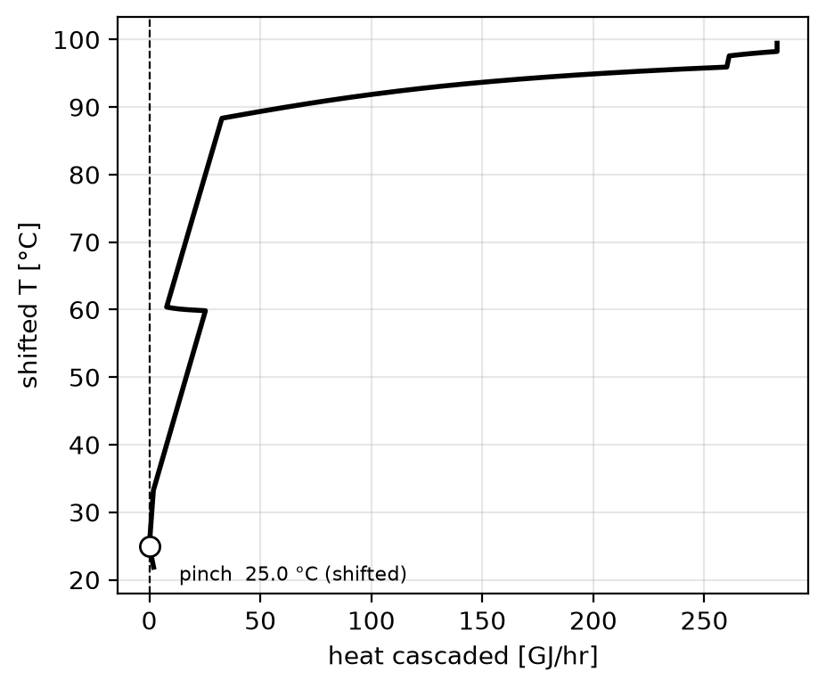
The grand composite curve: the heat cascaded through each shifted grid temperature once the minimum hot utility is supplied, plotted against that shifted temperature. Each boundary contributes two values, the heat arriving at it and the heat leaving it after its point loads, so a point load would appear as an exactly horizontal step. This system has none: the near-horizontal step near 60 °C shifted is the column condenser, whose glide spans about half a Kelvin, 65.4 to 64.9 °C on the real scale and 5 K lower on the shifted one – the same load that steps the hot composite curve at the corresponding real temperature. The curve touches zero exactly at the pinch, 298.15 K on the shifted scale, marked with an open circle, and continues below it to the bottom of the grid, 295 K. The value at the top of the curve is the hot utility supplied, 2.828e+08 kJ/hr, and the value at the bottom is the cold utility rejected, 1.936e+06 kJ/hr, small enough to be indistinguishable from zero on this axis. Touching zero is what makes further recovery impossible: no heat crosses the pinch.#
Targets versus the synthesized network#
The targets are a property of the streams alone. What the synthesized network of chapter 1 actually achieves is reported by the facility:
print(f'hot utility:  target {table.hot_util_load:.4g}, network {HXN.actual_heat_util_load:.4g} kJ/hr')
print(f'cold utility: target {table.cold_util_load:.4g}, network {HXN.actual_cool_util_load:.4g} kJ/hr')
# Those loads are utility-side (duty = unit_duty / heat transfer
# efficiency); the targets are process-side enthalpy differences, so
# sum the process-side duties of the network's utility exchangers too.
new_hus = [hu for hx in HXN.new_HX_utils for hu in hx.heat_utilities]
heat = sum(hu.unit_duty for hu in new_hus if hu.unit_duty > 0)
cool = -sum(hu.unit_duty for hu in new_hus if hu.unit_duty < 0)
print(f'hot utility,  process side: target {table.hot_util_load:.4g}, network {heat:.4g} kJ/hr')
print(f'cold utility, process side: target {table.cold_util_load:.4g}, network {cool:.4g} kJ/hr')
print(f"synthesis status: {HXN.synthesis_info['status']}")
hot utility:  target 2.828e+08, network 2.977e+08 kJ/hr
cold utility: target 1.936e+06, network 1.936e+06 kJ/hr
hot utility,  process side: target 2.828e+08, network 2.828e+08 kJ/hr
cold utility, process side: target 1.936e+06, network 1.936e+06 kJ/hr
synthesis status: mer
The first four lines are two different comparisons, and the difference between them
is not a property of the network at all. The first pair uses
HXN.actual_heat_util_load and HXN.actual_cool_util_load, which sum the
duty of each new utility exchanger’s HeatUtility. That is the
utility-side duty: biosteam defines duty as the exchanger’s process-side
duty divided by the utility agent’s heat-transfer efficiency, so it includes
the heat the agent loses on the way in. The second pair sums unit_duty
instead – the process-side duty of the same exchangers – which is the
quantity the problem table computes, an enthalpy difference of the process
streams themselves.
Compared like with like, on the process side, the network reaches both targets exactly: 2.828e+08 kJ/hr of hot utility and 1.936e+06 kJ/hr of cold utility, against targets of 2.828e+08 and 1.936e+06 kJ/hr. The utility-side heating figure, 2.977e+08 kJ/hr, is that same target divided by the heat-transfer efficiency of biosteam’s low-pressure steam agent, which is below one; it is the steam the plant must raise, not heat the network failed to recover. The cold utility needs no such correction, because the cooling agents used here (chilled and cooling water) have an efficiency of one, and both of its lines read 1.936e+06 kJ/hr.
The last line says the same thing in one word: the synthesis reports
HXN.synthesis_info['status'] as mer because the utilities of the network
it realized equal these targets. That is by construction rather than by luck.
The synthesizer plans each side of the pinch from the pinch outward on the
same stream curves this table was built from, so its own cascade is this
table, and it reaches the targets whenever its search finds a network without
stream splits that does (Key Concepts describes the planner). Where the
pinch design rules prove that the targets need a stream split, which hensmith
does not make, the status is best_effort and the network lies slightly
above the targets instead; Configuring the network and a larger system shows both outcomes on this
system.
Both directions of that statement are checked by the test suite, on the
process side. tests/test_hxn_mer.py synthesizes 40 problems for which an
unsplit MER network is known to exist and requires every one of them to reach
its targets and report mer, and 38 problems that provably need splits,
which must never beat their targets and must report best_effort.
tests/test_hxn_regression.py compares with its actual_loads helper,
which sums unit_duty exactly as the second pair of lines above does. It
synthesizes ten synthetic systems of increasing complexity and requires of
each synthesized network that it close its energy balance, that it never beat
the MER targets of the problem table computed on the same streams (and report
mer exactly when it reaches them), that it keep T_min_app inside every
exchanger, and that it recover at least as much heat as recorded in the test
file. A network that beat its target would be reporting an infeasible design;
a network that fell short of a recorded result would be a silent regression
in the synthesizer.
Where to next#
Anatomy of a synthesized network – the exchangers, stream life cycles and pinch temperatures behind the diagram, unit by unit.
Configuring the network and a larger system – what changing
T_min_appdoes to the targets and to the cost of reaching them.Key Concepts – the pinch concepts and terminology used throughout.